
Standalone photovoltaic (PV), wind, and battery systems offer a technically relevant architecture for electricity provision when grid supply is unavailable or unsuitable. Their design involves several interacting decisions: installed generation capacity, storage energy capacity, operational reserve, replacement timing, and acceptable unmet demand. Minimizing equipment cost alone can select a system with inadequate supply, whereas pursuing very low unmet energy can require additional generation or storage. Manufacturing burdens and replacement requirements add a further dimension to these trade-offs.
The environmental burden of renewable electricity depends on production processes, equipment lifetime, yield, and the system boundary. Sherwani et al. review PV electricity assessment and show why manufacturing and energy inputs belong in the comparison of generation technologies [1]. Davidsson et al. examine wind-system LCAs and provide a complementary basis for treating equipment manufacture and system configuration explicitly [2]. These studies establish the relevance of life-cycle indicators; they do not provide a universal equipment coefficient transferable without qualification to every off-grid installation.
System-level consistency also matters. Turconi et al. demonstrate the influence of electricity-system modeling and allocation assumptions in a Danish case study [3]. Their work motivates explicit boundaries and attribution in the present assessment, rather than serving as evidence for battery inventory values or a specific uncertainty-handling algorithm.
Resource forecasting and design-stage environmental modeling have already been integrated. Aloui et al. combine Bayesian-regularized NARX forecasting, component-level life-cycle models, and genetic optimization with goal-attainment refinement for standalone microgrids in southern Tunisia [4]. The present work therefore does not claim invention of that architecture, of the four objectives, or of the genetic/local-search combination.
Earlier uncertainty-aware microgrid planning also predates this study. Narayan’s multidisciplinary framework combines resource scenarios, stochastic sizing, and an LCA module [5]. Consequently, a defensible contribution requires more than listing forecasting, simulation, and LCA as separate modules. It requires a fully specified uncertainty mechanism, a consistent reference simulation, an identifiable deterministic control, and a test of whether design choices actually change.
The research question is whether a conditional resource-forecast distribution changes the feasible design set and its cost/environmental trade-offs when all other inputs are held fixed. A second question concerns verification: can an evolutionary method and its local refinement reproduce the front of a finite, exactly enumerated design space? These questions can be answered without presuming that uncertainty-aware sizing always improves realized reliability or that hybrid optimization always outperforms NSGA-II.
The study makes four implementation and evaluation contributions. First, it constructs a probabilistic NARX pipeline with disjoint chronological roles for training, tuning, residual calibration, sizing, and external evaluation. Second, it propagates jointly sampled weather-error blocks through a dispatch model with separate charge and discharge efficiencies and an explicit hourly energy balance. Third, it compares deterministic and scenario-constrained sizing on a shared discrete decision space using exactly the same weather ensemble, equipment assumptions, and load definition. Fourth, it validates the optimizer against enumeration and supplies the raw source records, processed inputs, code, forecast outputs, full objective landscapes, and numerical diagnostics.
These contributions are deliberately bounded. The environmental implementation is component-based screening with disclosed proxies and assumptions. It is not an audited inventory for a commissioned Tunisian installation. The forecasting experiment is rolling one-hour-ahead retrospective evaluation on gridded products, rather than an unconditional forecast of a future project lifetime. The load is a synthetic benchmark. These distinctions define the scope of the evidence instead of being deferred to unspecified supplementary material.
Section 2 positions the methods against relevant literature. Section 3 defines forecasting, dispatch, impact aggregation, and optimization. Section 4 documents the source data and numerical assumptions. Section 5 presents computed outcomes and verification. The remaining interpretive limits are discussed throughout the manuscript, and Section 6 states the supported conclusions.
ISO 14040 identifies the goal-and-scope, inventory, impact-assessment, and interpretation phases of LCA [6]. ISO 14044 provides requirements and reporting guidance for those phases [7]. In the present work, these principles motivate disclosure of the functional unit, equipment boundary, and data quality. Merely citing the standards is not treated as proof that the screening inventory satisfies every requirement of a comparative ISO-compliant LCA.
Technology-specific inventories should retain their applicable scope. Bonou et al. assess onshore and offshore wind technologies [8]; their findings support attention to infrastructure and equipment, but are not used here as a battery reference or as a direct numerical inventory for small wind turbines. The IEA PVPS inventory report documents material and energy flows for PV technologies and their balance of system [9]. It illustrates the information required for a detailed follow-on inventory, including technology and manufacturing geography.
Design-stage assessment is also relevant to electrification projects. Martínez-Rodríguez et al. apply an early-planning life-cycle framework to an off-grid project in Honduras [10]. Their case supports the usefulness of identifying material and construction hotspots before procurement. Its numerical outcomes are not transferred to the Kebili benchmark, whose equipment scope and demand assumptions differ.
NSGA-II provides non-dominated sorting and crowding-based diversity preservation [11]. These mechanisms are used as established search components rather than claimed as new algorithms. Coello Coello et al. discuss evolutionary multi-objective optimization, including local search and evaluation issues [12]. Their framework motivates reporting a reference front, objective scaling, evaluation budgets, and independent seeds when assessing hybrid refinement.
Abbes et al. investigate PV/wind/battery sizing with cost, supply-loss, and embodied-energy criteria [13]. The study also reports small-turbine embodied-energy estimates. One such reported coefficient is retained only as a screening proxy in the input registry; the present work does not imply that a generic turbine power curve reproduces the detailed performance or complete installed inventory of that reported product.
Bayesian regularization and stochastic dropout are distinct procedures. MacKay’s evidence-based regularization formulation provides an established treatment of regularization and model comparison [14]. The executable network in this study instead uses a fixed L2 penalty, training-time dropout, and Adam updates. No unsupported assertion is made that the implementation estimates evidence-based regularization hyperparameters.
Gal and Ghahramani provide a theoretical interpretation of dropout training as approximate Bayesian inference [15]. Here dropout masks generate model perturbations, while independently calibrated residual blocks represent additional forecast error. Kendall and Gal distinguish epistemic and aleatoric uncertainty [16]; this distinction is conceptually useful, but the residual-plus-dropout construction is not claimed to deliver an exact identifiable decomposition of the two sources.
Pinson and Girard emphasize that weather/power scenarios require attention to temporal interdependence, beyond marginal distributions at individual lead times [17]. This motivates shared multivariate residual blocks and masks held fixed within a scenario. Lahiri describes resampling methods for dependent observations [18], providing a methodological basis for block resampling while also making clear that block length is a substantive modeling choice.
Table 1 separates established components from the implementation choices being evaluated. The novelty is the traceable conditional-scenario experiment and its verification, not a priority claim for uncertainty-aware LCA in general. A measured-load, equipment-specific follow-on study would be needed to assess procurement decisions for a real community.
| Aspect | Established basis | Present implementation and test |
|---|---|---|
| Forecasting | NARX resource forecasting and probabilistic neural inference | Chronological training/tuning/calibration; rolling test scores and empirical prediction intervals. |
| Sizing | Multi-objective resource-based design and evolutionary search | Shared mean-trajectory control; explicit finite-scenario reliability constraint. |
| Environmental assessment | Component inventories and design-stage LCA | Independent GHG and energy coefficients with transparent screening scope. |
| Optimization verification | Non-dominance, diversity, and local refinement | Integer neighborhood refinement; five-seed comparison against exact enumeration. |
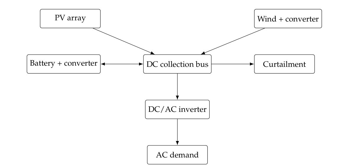
The hourly model connects PV generation, wind generation, and a battery to a DC collection bus, with an inverter supplying AC demand. Inverter power capacity is assumed sufficient for the benchmark load peak. Renewable surplus is curtailed when the battery cannot accept it. Converter parasitics, overload dynamics, voltage behavior, and switching transients are excluded. Figure 1 identifies the power-flow reference points; inverter losses occur once at the DC-to-AC delivery boundary.
The sizing experiment uses a transparent temperature-corrected power model rather than claiming execution of an uncalibrated single-diode/MPPT simulator. The array rating \(P_{\mathrm{PV,r}}\) is in kW, irradiance \(G_t\) in W/m\(^2\), and temperature in degrees Celsius:
The modeled array is horizontal, matching the downloaded zero-inclination radiation input. No GHI-to-tilted-plane transposition is silently applied. The DC loss factor aggregates soiling, mismatch, and wiring as a declared assumption; inverter efficiency is excluded from Eq. (2). Detailed PV performance models, such as the Sandia framework, require additional equipment and installation information [19]. Thus, this reduced model is suitable for the stated screening experiment but is not independent validation of a particular module.
Wind at 10 m is extrapolated to the assumed 30-m hub using
For one generic 3-kW turbine, the DC-equivalent power curve is
Total wind output is \(N_{\mathrm{WT}}p_{\mathrm{WT},t}\). The curve is explicitly generic: it is not a manufacturer-certified curve, and no site-calibrated roughness or turbulence adjustment is available. Rated, cut-in, and cut-out conditions are nevertheless implemented consistently, including zero output above cut-out.
Let \(e_t\) be stored energy in kWh and \(E_B\) nominal energy capacity. The DC demand is \(d_t=L_t/\eta_{\mathrm{inv}}\), with \(L_t\) the AC load in kW. Renewable supply is \(r_t=P_{\mathrm{PV},t}+N_{\mathrm{WT}}p_{\mathrm{WT},t}\). At each one-hour interval, charging and discharging obey
Only one of \(P_{\mathrm{ch},t}\) and \(P_{\mathrm{dis},t}\) is positive in an interval. The energy update is
Charging efficiency multiplies incoming energy, while discharging efficiency divides internal energy removal. This distinction prevents the energy-accounting error associated with multiplying both directions by the same efficiency. The battery power limit is \(P_{B,\max}=0.5E_B\) kW in the benchmark. No float-charging claim is made for the modeled lithium-ion proxy, and charging-control transients are excluded.
AC energy served and curtailment are calculated from the same dispatch:
Every hour is checked against the DC conservation identity
The annual trajectory is replayed until initial and final stored energy agree within \(10^{-8}\) kWh. Reported yearly totals use the final replay only. This periodic-state boundary avoids treating an arbitrary initial battery charge as a free annual energy source.
Annual equivalent full cycles are based on internal discharge throughput, not on all load energy:
Zero throughput gives an infinite cycle-limited lifetime; calendar life still applies. A zero-capacity battery contributes zero inventory and cost. Replacements occur at positive multiples of \(\tau_B^{(s)}\) strictly before the 20-year horizon. The proxy imposes a service-life ceiling and a throughput threshold, but does not model gradual capacity fade, temperature-dependent ageing, or depth-specific damage. It is used for comparative screening, not to predict a particular battery’s warranted life.
The physical reporting functional unit is one kWh of AC electricity delivered. Optimization retains absolute 20-year GHG and embodied-energy burdens as separate objectives, while delivered-energy intensities are reported as derived quantities. An absolute burden and an intensity are not interchangeable.
The implemented inventory covers aggregate initial PV, wind, battery, and inverter equipment, plus battery and inverter replacements. Component GHG coefficients \(g_j\) and energy coefficients \(a_j\) are independent inputs:
Here \(q_j\) uses the reference quantity of the coefficient: kW for PV, turbine count for wind, kWh of nominal battery capacity for storage, and unit count for the inverter. No generator GHG intensity per delivered kWh is added on top of these equipment factors. Embodied energy is not calculated as a fixed multiple of GHG.
The battery GHG proxy of 83.5 kg CO\(_2\)-eq/kWh is the midpoint of the 61–106 kg CO\(_2\)-eq/kWh production range reported by Emilsson and Dahllöf [20]. The transfer from vehicle-battery production to a generic stationary-storage proxy is disclosed. It is not an equipment-specific stationary LCI. The remaining assumptions and the small-wind energy proxy are identified in Table 4 and in the machine-readable registry.
Site transport, installation materials, foundations, recycling benefits, and waste treatment are not separately quantified. They are not hidden inside invented stage percentages. Environmental outputs are therefore described as life-cycle screening estimates, with component and initial/replacement decomposition. A complete cradle-to-grave extension requires procurement-specific inventories and treatment of these omitted stages. No Ecoinvent extraction or IPCC-2021 characterization run is claimed for the present execution.
The forecast target is \(\mathbf y_t=[G_t,v_{10,t},T_{a,t}]\). The model produces rolling one-hour-ahead predictions from six preceding observations of all three targets and five deterministic time/geometry features: sine and cosine of hour, sine and cosine of day of year, and sine of solar elevation. These 23 inputs are available without using contemporaneous or future weather targets. Solar elevation is an astronomical feature, not a measured future irradiance input.
One shared network has 48 tanh hidden units and three linear outputs. Training uses dropout probability 0.10, an L2 penalty of \(10^{-4}\) on weight matrices, Adam learning rate \(10^{-3}\), and batches of 256. Scaling statistics use the training period only. Early stopping selects the lowest tuning-year standardized MSE, with patience 12 and a maximum of 100 epochs. The selected weights are then frozen before residual calibration, sizing, and external evaluation. This implementation is explicitly dropout-regularized NARX, rather than an evidence-updated Bayesian-regularization implementation.
Calibration residual vectors are calculated using the frozen model on the separate 2021 year. For scenario \(s\), one stochastic dropout mask is held fixed across its entire trajectory, while multivariate residual blocks are sampled jointly:
The projection \(\Pi_t\) enforces nonnegative irradiance and wind, caps irradiance at 1400 W/m\(^2\) and wind at 60 m/s, and sets irradiance to zero at nonpositive solar elevation. Temperature is not artificially truncated. Residual blocks begin at midnight and are drawn from the same calendar quarter as the target block. A single sampled block supplies all three errors, preserving their joint relationship within the block. Independent random streams control masks and residual selection, so block-length comparisons hold the mask realizations fixed.
The base block length is 24 h; 72-h and 168-h blocks are evaluated separately. The construction preserves observed calibration dependence within sampled blocks, while transitions between blocks can disrupt longer persistence. It is not claimed to reproduce every multivariate climatological extreme. Dropout is an approximate model-perturbation mechanism, and residual errors contain observation-product, model, and structural contributions that cannot be separated exactly here.
The 5th and 95th sample quantiles define empirical 90% prediction intervals. These are prediction intervals for future product values, not confidence intervals for a mean and not confidence bounds on lifetime reliability. Forecast evaluation uses RMSE, MAE, \(R^2\), empirical coverage, mean interval width, CRPS, and the interval score. Gneiting and Raftery provide the proper-scoring framework for assessing predictive distributions [21]. Interval quality is reported even when coverage is conservative rather than exactly nominal.
The sizing year is 2022. Its scenarios are conditional retrospective trajectories: each hour’s input contains the preceding product values that would be known in rolling operation. They are not recursively generated unconditional future weather years. No 2023 value is used to construct the design scenarios or choose a configuration.
Twenty equally weighted trajectories define the base sizing distribution, \(p_s=1/20\). No scenario reduction or undocumented reweighting is applied. For the deterministic control, the weather input is exactly their pointwise mean, \(\overline{\mathbf y}_t=\sum\limits_s p_s\widetilde{\mathbf y}_t^{(s)}\). The simulator evaluates this mean trajectory separately; averaging simulated performance would be a different operation because dispatch and equipment conversion are nonlinear.
Scenario-specific objectives are
The scenario formulation minimizes
subject to \(\max_s\mathrm{LPSP}^{(s)}\leq0.05\). The deterministic formulation uses the corresponding four objectives and constraint for the mean trajectory. Shapiro et al. provide the general scenario-based stochastic-programming context [22]. The implemented maximum is a finite-scenario constraint; it is not a chance constraint or a guarantee for all possible future weather.
The quantity traditionally labeled LPSP is defined here as an unmet-energy fraction:
It is not the probability that any outage occurs. The 5% threshold refers to annual demand energy and does not limit individual outage duration. All candidates are subject to the same synthetic annual load.
For project horizon \(Y\), real discount rate \(r\), replacement times \(\tau_{jk}^{(s)}\), and zero salvage in the benchmark,
The denominator is served electricity, not total renewable production. Fractional replacement times are discounted at their modeled time. Each sizing trajectory is assumed to represent a stationary annual replay over the project lifetime; no 20-year weather forecast or annual PV degradation trend is implied. Environmental burdens and their physical delivered-energy denominator are not economically discounted.
The decision vector is \(\mathbf x=(P_{\mathrm{PV,r}},N_{\mathrm{WT}},E_B)\). The finite set contains PV ratings 0–8 kW in 0.5-kW increments, 0–2 turbines of 3 kW each, and battery capacities 0–24 kWh in 2-kWh increments. All 663 combinations are evaluated. Designs with zero generation may be evaluated for completeness but cannot satisfy the supply constraint.
Enumeration gives the exact feasible Pareto set on this declared grid. It does not certify a continuous-capacity optimum. NSGA-II and HGA are subsequently tested on the same cached objective landscape without receiving the reference front. Both have population 40 and budget 800 objective calls per seed; repeated designs still count as calls. Five seeds are fixed before comparison.
The integer NSGA-II implementation uses feasibility-first comparison, non-dominated sorting, crowding distance, binary tournaments, uniform crossover, and bounded integer mutations. HGA uses 720 evolutionary calls and reserves 80 for local refinement. Up to five promising feasible points define starting designs. The goal and weights are obtained from the discovered front, not from enumeration. Local refinement minimizes
by feasible one-step integer coordinate neighborhoods. This is an explicit mixed-integer goal-attainment adaptation, avoiding continuous local steps that would silently violate equipment counts.
Quality is assessed by reference-front recovery and normalized inverted generational distance (IGD) to the enumerated front. Normalization uses the range of the feasible objective landscape for evaluation only. Both search methods use the same evaluation budget. Cached-objective search timing is not presented as end-to-end simulation speed. An algorithmic advantage is claimed only if the observed quality comparison supports it.
Nominal performance means simulation under the mean weather trajectory; expected performance means the weighted mean of scenario-specific outcomes; objective-specific worst performance means the maximum of that particular objective over scenarios. The scenario maximizing LPSP need not maximize cost or an environmental objective. Selected designs are also replayed on the unused 2023 reference weather. This external-year evaluation is reported separately from design-scenario feasibility.
Environmental inventories can remain identical across scenarios for a fixed design when replacement counts do not change. In that situation, uncertainty influences absolute burdens through the selected configuration, not through a spurious variation of manufacturing emissions with weather. Delivered-energy intensities may still vary with energy service. The reporting distinguishes these pathways explicitly.
The spatial query is Kebili, southern Tunisia, at 33.7\(^\circ\)N, 8.97\(^\circ\)E; the returned elevation is 40 m. This identifies a gridded resource location, not a named instrumented weather station or an observed household. The load is a engineering benchmark with a morning bump, an evening bump, and a modest seasonal term. For hour \(h_t\) in UTC+1 and local day of year \(d_t\), the unscaled profile is
It is normalized independently in each evaluation year to 6000 kWh. The 2022 peak is 1.622 kW. The chosen shape and annual magnitude are assumptions, not a fitted survey of Tunisian households. They are held constant in definition across sizing approaches, enabling a controlled comparison while limiting generalization to a real community.
PVGIS version 5.3 supplies hourly radiation and meteorological products through the European Commission Joint Research Centre’s documented API [23]. The actual downloaded metadata identify PVGIS-SARAH3 radiation and ERA5 meteorology. The query requests zero panel inclination, explicit coordinates, one calendar year at a time, and JSON output. Retrieved raw JSON files are preserved with SHA-256 hashes and exact queries.
The six years contain 52,584 records, including 8784 hours in leap year 2020. Variables are global radiation on the requested horizontal plane, 10-m wind speed, 2-m air temperature, solar elevation, and the provider’s radiation-reconstruction flag. No missing variable values, duplicate hourly slots, negative irradiance, negative wind, or radiation-reconstruction flags occur in the retrieved records. No interpolation or artificial gap filling is performed.
Provider timestamps retain their original minute offsets in the archive and processed CSV. For dispatch, each record is assigned to its nominal UTC hourly slot; source values are retained unchanged. Treating reported radiation as an hourly mean for energy integration is a model convention. The source products are satellite/reanalysis estimates, so forecast accuracy against them is not equivalent to validation against a local radiometer or anemometer.
Table 2 specifies every chronological role. The six initial lag hours reduce the 2018–2019 training count to 17,514. At later year boundaries, only preceding already-available observations supply lag history. No random reassignment mixes future target years into training. The 2020 tuning year selects the trained model; 2021 supplies forecast-error calibration; 2022 supports sizing; 2023 is reserved for forecast and design evaluation.
| Role | Years | Target hours |
|---|---|---|
| Training | 2018–2019 | 17,514 |
| Tuning / model selection | 2020 | 8,784 |
| Residual calibration | 2021 | 8,760 |
| Sizing | 2022 | 8,760 |
| External evaluation | 2023 | 8,760 |
Table 3 provides the executable engineering and financial assumptions. All monetary coefficients are constant USD-denominated benchmark values, rather than supplier quotes or estimates of current Tunisian procurement prices. A real discount rate of 8% and 20-year horizon define the base case. Replacement batteries retain the same unit capital cost, and inverter replacement occurs at year 10. Salvage, decommissioning cost, and inflation are zero in this benchmark and must be reconsidered for investment appraisal.
| Category | Parameter | Value |
|---|---|---|
| PV | NOCT; temperature coefficient; DC loss | 45 \(^\circ\)C; \(-0.004\) K\(^{-1}\); 10% |
| Wind | Rated power; cut-in / rated / cut-out | 3 kW; 3 / 12 / 25 m/s |
| Wind height | Hub height; shear exponent | 30 m; 0.14 |
| Battery | Charge / discharge efficiencies | 0.95 / 0.95 |
| Battery | SOC limits; power limit | 10–95%; 0.5 kW per nominal kWh |
| Battery service | Calendar ceiling; discharge EFC limit | 10 years; 3000 EFC |
| Inverter | Efficiency; life | 0.96; 10 years |
| Demand / reliability | Annual demand; energy-loss limit | 6000 kWh; 5% |
| Project | Horizon; real discount rate | 20 years; 8% |
| Capital costs | PV; wind; battery; inverter | 1200 USD/kW; 7500 USD/turbine; 400 USD/kWh; 1500 USD/unit |
| Annual O&M | PV; wind; battery fractions | 1%; 2%; 1% of component capital cost |
| Excluded cost terms | Salvage; decommissioning; inflation | Zero in the benchmark |
The battery has zero self-discharge in this implementation. Costs are not dated market quotations. No PV or wind replacement is imposed within 20 years.
Table 4 keeps reference quantities, units, and provenance visible. The PV, wind-GHG, battery-energy, and inverter coefficients are explicit analyst screening assumptions. The battery GHG midpoint and turbine-energy proxy are literature-anchored transfers with the limitations already described. A machine-readable input registry records these distinctions, preventing assumed values from being presented as licensed database extractions or measured project inventory.
| Component / unit | GHG (kg CO\(_2\)-eq) | Energy (MJ) | Provenance and transfer limit |
|---|---|---|---|
| PV / kW | 700 | 8000 | Analyst screening assumptions; not an equipment-specific database extraction. |
| Wind / 3-kW turbine | 2500 | 19504.738 | GHG is an assumption. Energy is the reported Wind 3000 proxy from Abbes et al. [13]; generic performance curve and incomplete installed boundary. |
| Battery / kWh | 83.5 | 1000 | GHG is the midpoint of a vehicle-battery production range [20], transferred to stationary storage. Energy is an independent assumption. |
| Inverter / unit | 200 | 2500 | Analyst screening assumptions; initial unit and year-10 replacement. |
Reference quantities are nominal capacities or unit counts, not delivered electricity. Transport, site works, and end-of-life processes are not separately inventoried.
The annual operation-and-maintenance fractions are 1% of PV capital cost, 2% of wind capital cost, and 1% of battery capital cost. Battery replacement follows Eq. (11); an inverter has a 10-year benchmark life. PV and wind equipment are not replaced inside the 20-year horizon. This simplifying lifetime assumption should not be read as a warranty statement. Costs are conditional on the declared capacity grid and load, and no currency conversion or market-price forecast is used.
Zero wind and zero storage are admissible choices; the optimization is not forced to install every technology. This enables the result to show whether wind is preferred under the available resource and screening assumptions. The grid resolution is an engineering approximation. Enumeration verifies only these choices, while commercial module strings, inverter sizing, and discrete battery products would require a procurement-specific feasible set.
The base sizing set contains 20 conditional 2022 trajectories with equal weights. A nested pool of 40 trajectories supports 5-, 10-, 20-, and 40-scenario checks. The predictive-interval evaluation uses 100 independent 2023 samples. Scenario weights and seeds are retained, and no quantile selection or undocumented representative-day compression is used.
One-at-a-time sensitivity changes the discount rate, selected costs, impact coefficients, cycle limit, and calendar life by \(\pm20\%\), recomputing the entire feasible Pareto front. Residual-block length is separately varied while holding dropout-mask draws fixed. These are local screening analyses. They identify responses within tested ranges but do not establish global variance contributions, interactions, or universal parameter dominance.
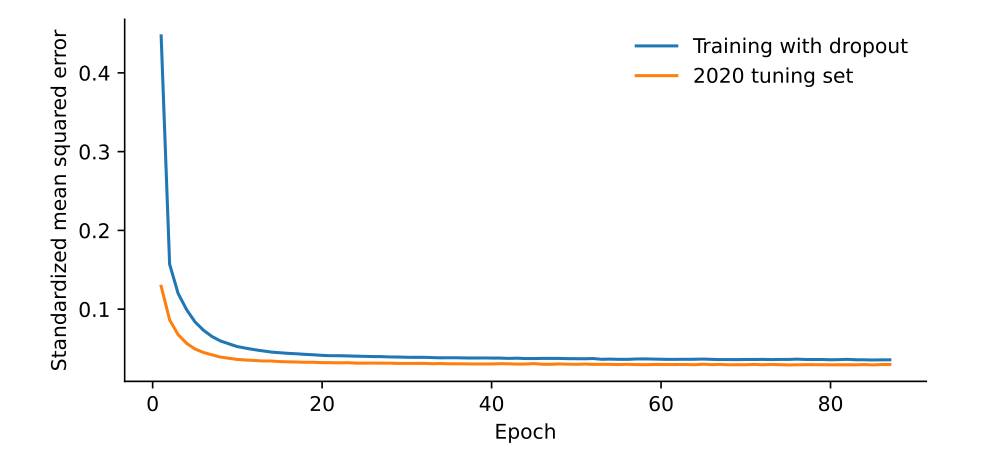
Training stops after 87 epochs, and epoch 75 has the lowest tuning-year error. Figure 2 shows the recorded training and tuning losses; training-time dropout makes the two loss curves different evaluation conditions. The 2021 residual correlations are weak for irradiance–wind (0.035), small for irradiance–temperature (0.084), and negative for wind–temperature (\(-0.169\)). Joint residual sampling retains these observed pairings instead of presuming independent weather errors.
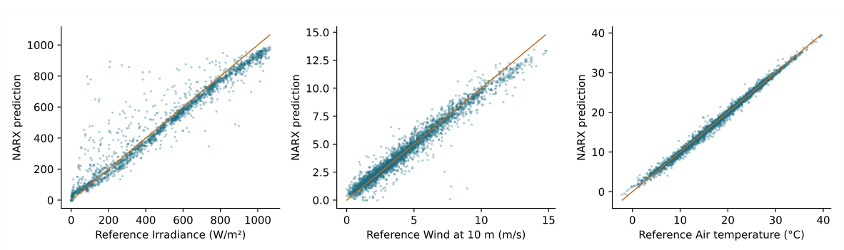
Table 5 reports point accuracy against the unused 2023 product values. Relative to persistence, RMSE decreases by 58.00%, 17.48%, and 57.83% for irradiance, wind, and temperature. These are paired comparisons on the same hourly records, rather than comparisons across different datasets. Figure 3 makes the remaining scatter visible. No superiority over every forecasting family is asserted: recurrent networks, quantile models, and independently tuned probabilistic baselines have not been benchmarked.
| Variable | NARX RMSE | NARX MAE | \(R^2\) | Persistence RMSE |
|---|---|---|---|---|
| Irradiance (W/m\(^2\)) | 47.994 | 19.072 | 0.9784 | 114.269 |
| Wind at 10 m (m/s) | 0.496 | 0.326 | 0.9572 | 0.601 |
| Air temperature (\(^\circ\)C) | 0.565 | 0.397 | 0.9963 | 1.341 |
Persistence uses the preceding hour, with the same physical night projection for irradiance. RMSE and MAE have the units shown in the first column.
Percentage errors need a defined denominator. Irradiance MAPE is 17.26% on 4155 hours with reference irradiance above 20 W/m\(^2\); wind MAPE is 11.38% on 8634 hours above 0.5 m/s. Temperature MAPE is 0.135% using absolute temperature in kelvin, rather than dividing by Celsius values near zero. MAE in degrees Celsius remains the more direct temperature error measure. These exclusions and units prevent night zeros or an arbitrary Celsius origin from producing misleading percentage comparisons.
Table 6 evaluates the predictive distribution separately from point accuracy. Daylight irradiance and all-hour wind coverage exceed the nominal 90% level moderately; temperature coverage of 98.29% indicates appreciable over-dispersion. The interval scores and CRPS penalize unnecessary spread as well as missed observations. The residual-plus-dropout construction should therefore be regarded as a tested approximate scenario mechanism, not as proof of exact uncertainty calibration. Nighttime irradiance intervals collapse to zero by physical projection and are excluded from daylight coverage to avoid inflating that assessment.
| Variable | Hours | Coverage (%) | Width | CRPS | Interval score |
|---|---|---|---|---|---|
| Irradiance | 4,293 | 92.92 | 197.119 | 27.030 | 308.224 |
| Wind at 10 m | 8,760 | 91.61 | 1.514 | 0.238 | 2.140 |
| Air temperature | 8,760 | 98.29 | 2.872 | 0.312 | 3.058 |
Irradiance scores use daylight (\(H_{\mathrm{sun}}>0\)); wind and temperature use all hours. Width, CRPS, and interval score have each variable’s physical units. Lower scores are preferable; nominal coverage is 90%.
The complete grid contains 210 deterministic-feasible and 186 scenario-feasible configurations, with 11 and 24 non-dominated configurations, respectively. Each front is exact on the declared capacity grid. Figure 4 shows two objective projections while encoding the relevant reliability objective; a plotted projection alone does not define dominance in all four dimensions.
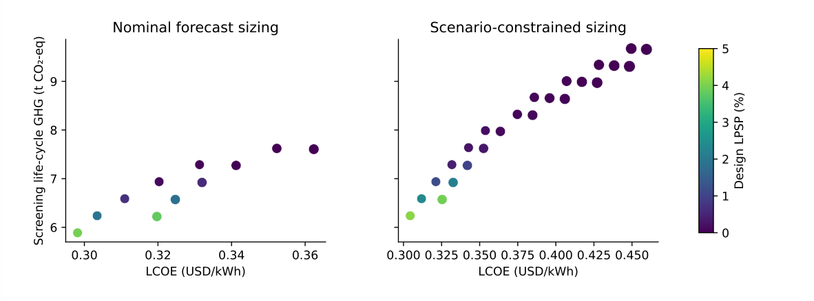
All base-case Pareto configurations select zero wind. This is an optimization outcome under the downloaded wind product, generic power curve, load, and screening coefficients, rather than a restriction requiring a PV-only solution. It does not establish that small wind is unsuitable for other sites or that a certified local turbine would have the same economics.
Table 7 identifies distinct configurations rather than independently combining favorable objective values from different designs. The least-cost deterministic design uses 4.5 kW PV and 14 kWh battery. The scenario-constrained least-cost design uses 5.0 kW PV with the same battery capacity, an 11.1% PV increase and a 2.10% increase in its reported LCOE. Its absolute screening GHG increases from 5888 to 6238 kg CO\(_2\)-eq, and embodied energy from 69000 to 73000 MJ. Under these factors, the same least-cost configuration also minimizes both environmental burdens; the other low-GHG/low-energy rows are explicitly labeled alternatives, not separate global minima.
Table 8 presents the nominal performance, scenario-mean performance, objective-specific maximum performance, and external performance of the two least-cost designs.
| Form / selection | PV | WT | Battery | LCOE | LPSP | GHG | EE |
|---|---|---|---|---|---|---|---|
| D / Least cost | 4.5 | 0 | 14 | 0.2981 | 3.954 | 5888 | 69.0 |
| D / Low GHG | 4.5 | 0 | 16 | 0.3197 | 3.801 | 6222 | 73.0 |
| D / Low energy | 5.0 | 0 | 14 | 0.3035 | 1.952 | 6238 | 73.0 |
| D / Balanced | 5.5 | 0 | 14 | 0.3110 | 0.721 | 6588 | 77.0 |
| UA / Least cost | 5.0 | 0 | 14 | 0.3044 | 4.127 | 6238 | 73.0 |
| UA / Low GHG | 5.0 | 0 | 16 | 0.3254 | 3.942 | 6572 | 77.0 |
| UA / Low energy | 5.5 | 0 | 14 | 0.3118 | 2.349 | 6588 | 77.0 |
| UA / Balanced | 6.0 | 0 | 14 | 0.3212 | 1.185 | 6938 | 81.0 |
D: deterministic; UA: uncertainty-aware. PV is kW; WT is the number of 3-kW turbines; battery is kWh; LCOE is USD/kWh; LPSP is percent; GHG is kg CO\(_2\)-eq; EE is GJ. D rows report mean-trajectory simulation; UA rows report mean LCOE/burdens and worst-scenario LPSP. Low-GHG/low-energy alternatives are the best remaining distinct choices in those rankings; the least-cost design also minimizes both burdens. The balanced row minimizes the maximum normalized objective departure over the front, after excluding previously selected rows.
| Design | Evaluation | LCOE | LPSP (%) | GHG (kg) | EE (GJ) |
|---|---|---|---|---|---|
| D | Mean trajectory | 0.2981 | 3.954 | 5888 | 69.0 |
| D | Scenario mean | 0.2991 | 4.265 | 5888 | 69.0 |
| D | Scenario maximum | 0.3075 | 6.874 | 5888 | 69.0 |
| D | External 2023 | 0.2995 | 4.395 | 5888 | 69.0 |
| UA | Mean trajectory | 0.3035 | 1.952 | 6238 | 73.0 |
| UA | Scenario mean | 0.3044 | 2.245 | 6238 | 73.0 |
| UA | Scenario maximum | 0.3103 | 4.127 | 6238 | 73.0 |
| UA | External 2023 | 0.3050 | 2.443 | 6238 | 73.0 |
D installs 4.5 kW PV and 14 kWh battery; UA installs 5.0 kW PV and 14 kWh battery. Both have zero wind. LCOE is USD/kWh; GHG is kg CO\(_2\)-eq. Maximum values are calculated separately for each objective. They are finite-scenario extrema, not statistical confidence bounds.
Replaying the deterministic least-cost choice across the same scenario set yields maximum LPSP 6.874%, exceeding the 5% design constraint. The scenario-constrained choice reduces that maximum to 4.127%. This demonstrates a changed margin on the sampled design trajectories. It does not imply immunity to unobserved weather extremes.
The physical delivered-energy normalization gives 53.18 g CO\(_2\)-eq/kWh and 0.622 MJ/kWh for the uncertainty-aware least-cost configuration. These are ratios of mean total burden to 20 times mean annual served electricity under stationary replay. They are not discounted economic intensities. The full representative-intensity table is supplied in the results archive, while the optimization continues to use absolute burdens.
Every configuration on each base front meets the 5% unmet-energy criterion on the unused 2023 reference weather. The deterministic least-cost design has external LPSP 4.395%, compared with 2.443% for the scenario-constrained least-cost choice. Additional PV therefore lowers unmet energy in this year, but both already satisfy the threshold. A claim that uncertainty-aware sizing eliminates external-year violations would be unsupported by this experiment because neither front has a violation. One held-out weather year also cannot estimate the probability of a rare multi-year shortage.
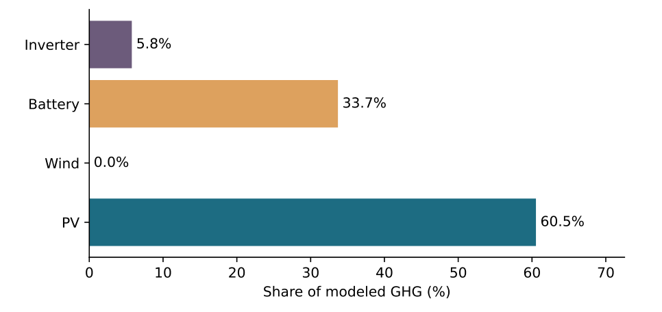
The uncertainty-aware balanced representative installs 6.0 kW PV and 14 kWh battery, with no wind. Its total modeled GHG is 6938 kg CO\(_2\)-eq. The exact decomposition is 4200 kg for PV, 1169 kg for the initial battery, 1169 kg for one battery replacement, and 200 kg each for the initial and replacement inverter. Their shares are 60.54%, 16.85%, 16.85%, 2.88%, and 2.88%, summing to 100% up to rounding. Figure 5 aggregates these stages by component.
The calendar ceiling gives one battery replacement in each base scenario for this configuration, so the absolute burden does not vary among its scenarios. Its uncertainty-related change arises through configuration selection and energy delivery. Changing the lifetime or coefficient assumptions can alter that result; the hotspot ranking is not a measured breakdown for installed equipment.
Minimum cost changes by approximately 0.06% between 20 and 40 scenarios, but the feasible count changes from 186 to 183 and the front from 24 to 25 configurations (Table 9). Minimum screening GHG and embodied energy remain unchanged. Cost stability therefore provides a limited check; it does not justify declaring the whole distribution or Pareto set converged.
| Scenarios | Feasible designs | Front size | Minimum LCOE |
|---|---|---|---|
| 5 | 186 | 22 | 0.30561 |
| 10 | 186 | 24 | 0.30496 |
| 20 | 186 | 24 | 0.30439 |
| 40 | 183 | 25 | 0.30420 |
All rows have minimum GHG 6238 kg CO\(_2\)-eqand minimum energy 73000 MJ. LCOE is USD/kWh. A small change in the minimum cost does not establish convergence of every Pareto configuration or rare-event reliability.
With the same 20 dropout-mask draws, 24-, 72-, and 168-hour residual blocks yield 186, 186, and 183 feasible configurations and fronts of 24, 16, and 21 configurations. Minimum LCOE remains approximately 0.3044 USD/kWh. The change in front membership demonstrates that temporal-error construction matters even when the minimum cost is almost unchanged. The test motivates further dependence validation rather than an assertion that a particular block length is universally correct.
Increasing battery unit cost by 20% raises the minimum front LCOE by 9.98%; increasing discount rate and PV cost by the same proportion raises it by 8.52% and 7.52%, respectively. Wind cost changes have no effect on the minimum in the tested range because the preferred configurations omit wind. Reducing the battery calendar ceiling from 10 to 8 years raises minimum LCOE by 11.79%, minimum GHG by 18.74%, and minimum embodied energy by 19.18%. Reducing the throughput limit from 3000 to 2400 EFC raises the corresponding minima by 9.93%, 10.71%, and 10.96%.
Independent coefficient changes produce interpretable environmental responses. A 20% increase in the PV GHG coefficient increases minimum GHG by 11.22%, while the same proportional battery coefficient increase produces 7.50%. The corresponding PV- and battery-energy changes increase minimum energy by 10.96% and 7.67%. These are re-optimized, one-at-a-time front minima, which can refer to different designs. They are not global sensitivity indices or simultaneous changes at one fixed configuration.
Figure 6 shows the changes in the minimum scenario-front LCOE resulting from a 20% increase in selected input parameters. The complete results for both positive and negative perturbations, including the corresponding environmental responses and resulting front sizes, are provided in the accompanying CSV file.
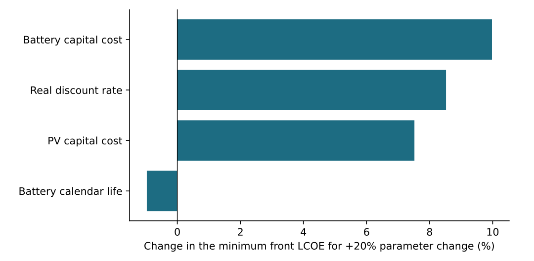
Table 10 compares five-seed, equal-budget search performance against the enumerated scenario front.
| Method | Seeds | Full recovery | Mean recovery (%) | Mean IGD | Unique designs |
|---|---|---|---|---|---|
| NSGA-II | 5 | 4 | 99.17 | 0.000178 | 214–253 |
| HGA | 5 | 3 | 98.33 | 0.000356 | 207–249 |
Population 40; 800 objective calls per seed. Repeated evaluations count toward the budget. Full recovery counts runs finding all reference-front configurations. IGD is normalized against the feasible landscape; lower is better. No inferential significance or runtime-superiority claim is made.
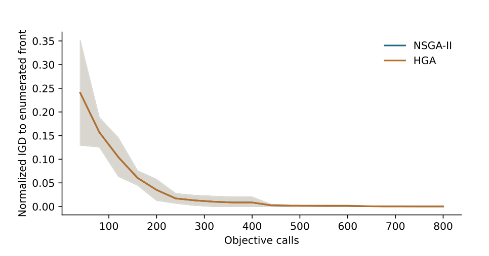
NSGA-II recovers the complete 24-configuration front in four of five runs; HGA does so in three of five. In each remaining run, one reference configuration is missed. Both methods recover the same minimum LCOE in all seeds. Mean recovery is 99.17% for NSGA-II and 98.33% for HGA, and normalized mean IGD is 0.000178 and 0.000356. These small-sample results provide no evidence of a hybrid quality advantage; the hybrid’s final completeness is slightly lower in this benchmark. No statistical significance is inferred from five runs.
Figure 7 presents the normalized IGD as a function of the actual number of objective-function evaluations. The lines represent the mean values across five independent seeds, while the shaded bands indicate one standard deviation. The enumerated feasible front is used as the reference set, with lower IGD values indicating better search performance.
Enumeration evaluates only 663 unique designs, fewer than each algorithm’s budget of 800 calls including repeats. On this finite benchmark enumeration is the more direct way to obtain a verified front. Evolutionary comparison evaluates implementation behavior; it does not establish a computational reason to replace enumeration here. Larger continuous or mixed-integer problems would require a separate scalability study.
All five independently specified analytical checks pass. The maximum hourly DC balance residual over the sizing pool is \(2.0\times10^{-15}\) kWh, and the maximum periodic-state residual is zero to the recorded numerical precision. Annual served plus unmet electricity reconciles with 6000 kWh demand. These results support conservation and implementation consistency, while leaving equipment realism and input validity as separate questions.
The integrated architecture overlaps substantially with Aloui et al. [4], so the present evidence should be assessed as an explicit conditional-scenario implementation and verified comparison. Differences in load, grid resolution, resource years, component models, inventory scope, and cost assumptions prevent a like-for-like numerical ranking against that study. No reproduced baseline from its proprietary or unpublished inputs is claimed.
The experiment supports three limited practical observations: sampled uncertainty can remove configurations that appear feasible under a mean trajectory; maintaining that sampled margin can require additional generation and screening burden; and local refinement does not necessarily improve an evolutionary front at a fixed budget. A procurement study should repeat the calculation with measured demand, equipment-specific performance, localized costs, and a defensible full inventory before selecting hardware.
This study executes an uncertainty-aware microgrid sizing framework using six years of traceable PVGIS-SARAH3/ERA5 input, a chronologically separated NARX experiment, joint forecast-error scenarios, energy-conserving dispatch, and independently parameterized environmental indicators. Enumeration verifies the declared finite design space, while an equal-budget comparison tests evolutionary and integer goal-attainment search.
Forecast uncertainty changes the admissible design set from 210 to 186 configurations under the base 5% unmet-energy criterion. The least-cost deterministic and scenario-constrained designs cost 0.2981 and 0.3044 USD/kWh, respectively, within the stated economic assumptions. The scenario-constrained least-cost choice adds 0.5 kW PV while retaining 14 kWh of nominal battery capacity. Both fronts meet the threshold in the unused 2023 reference year; the evidence therefore supports a changed design-scenario margin, rather than a demonstrated reduction in external-year threshold violations.
NSGA-II recovers the complete scenario front in four of five seeds and HGA in three of five. Both find the same minimum cost in every run; the final-quality results do not justify a superiority claim for hybrid refinement. Environmental trade-offs and hotspots are conditional on the disclosed screening factors and replacement model. The accompanying package makes the data, assumptions, complete objective landscapes, and validation checks inspectable, while identifying the equipment inventory and measured-demand work needed for a site-specific follow-on assessment.
This research received no external funding.
The author declares that there are no competing interests.
The data supporting the findings of this study are available from the author upon reasonable request.
Generative artificial intelligence tools were used solely for language editing, grammatical correction, and improvement of readability. The author reviewed and verified the final manuscript and assumes full responsibility for its accuracy, integrity, and scholarly content.