
Smart and functional materials change an engineering component’s role from passive load carriage to interaction with its environment. Piezoelectric phases transduce mechanical and electrical fields, piezoresistive composites change resistance under deformation, and shape-memory systems provide activated recovery. Additive manufacturing (AM) offers geometric freedom, internal architecture, and opportunities for localized functional integration. Gibson and colleagues describe the process capabilities that enable these manufacturing choices [1]. Their availability does not establish that a particular combination of host, functional phase, and manufacturing process is qualified for service.
Qualification becomes more demanding when functionality and structural integrity share the same geometry. The tomography-focused review by du Plessis and colleagues explains why defect size, morphology, and location provide information that bulk porosity alone cannot capture [2]. Sanaei and Fatemi review the consequences of these defects for fatigue performance and the limitations of nominal material-property descriptions [3]. Bartlett and Li address residual stresses in metal powder-bed fusion, providing a separate reason to connect process history with component response [4]. Together, these issues motivate an uncertainty model that distinguishes a manufacturing descriptor from a calibrated failure predictor.
Mechanical and functional performance can deteriorate differently. Fatemi and colleagues report processing- and loading-direction effects in fatigue experiments on AM Ti–6Al–4V [5]; these material-specific observations should not be transferred directly to another material system. Solberg and Berto discuss continuing challenges in fatigue assessment of AM metals [6]. A self-sensing structure introduces additional concerns: conductive-route interruption, host–sensor strain-transfer loss, temperature cross-sensitivity, calibration error, and baseline drift. A mechanically serviceable component can therefore become diagnostically unavailable, while a functioning sensor can remain attached to a component approaching a structural limit.
Geometry optimization provides one part of this problem. Bendsøe and Sigmund establish the mathematical foundations of topology optimization [7]. Zhu and colleagues discuss AM-specific opportunities and challenges, including the integration of material, structure, process, and performance [8]. The present benchmark does not perform topology optimization. It searches a finite parametric design set and asks how sensing and maintenance assumptions change the admissibility and economic ranking of its members.
Self-sensing AM lattices are an established research direction. Ubaid and colleagues experimentally and numerically investigated architected conductive-composite lattices with tunable structural and sensing properties [9]. Health-informed maintenance involving AM also has precedents: Cubillo and colleagues developed a cost and downtime model linking health monitoring, maintenance decisions, and AM repair opportunities [10]. The contribution here is narrower than the invention of either self-sensing or AM-enabled maintenance. It is a connection between defect-sensitive progression, deteriorating diagnostic information, uncertainty-aware replacement, and independently checked lifecycle reliability.
The study provides a complete computational benchmark with explicit assumptions and separate structural and diagnostic endpoints. It derives a distinguishable three-interrogation sensing model, propagates a latent fatigue rate through an approximate Gaussian estimator, and selects a design using confidence-based constraints. Code, all design-level outputs, and trajectory-level confirmation data accompany the manuscript. Numerical verification evaluates implementation consistency; experimental validation is identified separately and is not claimed.
For reliability engineering, the useful classification is the pathway by which a material produces a signal or action. Table 1 organizes possible mechanisms and corresponding degradation questions. These are alternative technology families rather than materials simultaneously represented in the bracket benchmark. Its specific numerical sensing mechanism is a normalized piezoresistive-like response with repeated calibration interrogation; actuation and functional authority are outside its scope.
| Family | Engineering opportunity | Degradation or qualification question |
|---|---|---|
| Piezoelectric phase | Conformal or embedded electromechanical sensing | Electrode integrity, depoling, interface durability, calibration stability |
| Piezoresistive composite | Printed strain- and damage-responsive routes | Conductive-network interruption, gain loss, hysteresis, thermal compensation |
| Shape-memory system | Activated geometry or stiffness change | Transformation fatigue, incomplete recovery, thermal compatibility |
| Functionally graded material | Spatial redistribution of properties | Gradient continuity, composition control, thermal mismatch |
| Architected cellular material | Geometry-dependent compliance and mass | Strut imperfections, local instability, notch sensitivity, size effects |
Functional integration can introduce competing design requirements. A compliant region can increase a measurable response while increasing local cyclic strain. A wide sensing route can improve durability while adding manufacturing effort. Additional routes can reduce independent measurement noise but cannot remove a disturbance common to every route. These interactions justify including sensor architecture and maintenance policy among the design variables.
The initial defect description is
where \(a_0\) is an equivalent initial flaw length, \(\eta_s\) increases with proximity to the surface, \(\chi\) describes morphology severity, \(\sigma_r\) is tensile residual stress, and \(R_a\) is a surface-roughness descriptor. Murakami’s treatment of small defects provides foundational context for separating a defect descriptor from a nominal strength value [11]. Zerbst and colleagues further distinguish crack initiation, short-crack development, long-crack propagation, and arrest [12]. The simplified growth model below omits initiation and arrest and must be interpreted accordingly.
In a calibrated application, a process vector \(\mathbf p=\{P,v,h_p,t_l,\theta\}\) could condition a distribution \(f(\mathbf d_0\mid\mathbf p,\mathbf y_{\mathrm{proc}})\) using build-monitoring evidence. Power, speed, hatch spacing, layer thickness, and orientation cannot be inferred from the present study. Only orientation and a binary finishing level enter its prescribed response maps. Surface roughness is represented indirectly through an assumed stress multiplier rather than an independently measured \(R_a\) distribution. Independent primitive uncertainty draws are used as a choice, not an assertion that actual AM process variables are independent.
The component has mechanical damage \(D_m\in[0,1)\) before structural-limit exceedance, fractional functional gain loss \(D_f\in[0,0.95]\), and signed normalized drift \(b\in\mathbb R\). Drift is not a monotonically increasing damage fraction. If a dimensionless severity is needed, \(D_s=|b|/b_{\mathrm{tol}}\) can be reported without restricting it to unity. The implemented evolution over a time step is
where \(Z_k\sim\mathcal N(0,1)\), \(v_m\) is a unit-specific fatigue progression rate, and \(\xi_f,\xi_b\) are mission-specific multipliers. The time unit is kilohours: \(1\,\mathrm{kh}=1000\) h. Mechanical deterioration increases the assumed gain-loss increment; gain loss and drift affect diagnostic information; the resulting information controls replacement. Replacement draws a new structural unit and resets its three states. These are the implemented coupling pathways, rather than an implicit claim that all underlying physical fields are solved together.
Paris and Erdogan provide the classical crack-growth relation underlying the benchmark’s propagation law [13]. For an assumed exponent of three and constant unit-specific forcing, the model is
with
Here \(\Delta\sigma\) is in MPa, \(a\) in m, \(C\) in \(\mathrm{m\,cycle^{-1}}(\mathrm{MPa}\sqrt{\mathrm m})^{-3}\), and \(\xi_e,\xi_L\) represent environment and load multipliers. The residual-stress multiplier \(M_r\), morphology map \(Y\), and environmental multiplier are analyst-defined assumptions. They are not calibrated Walker, closure, or material-specific mean-stress laws. The Paris exponent and coefficient distribution are also illustrative.
For \(a_c=0.8\) mm, integration gives
Thus \(D_m\) progresses linearly in cycles for this transformed crack coordinate, while \(a\) grows nonlinearly. The structural endpoint is the first crossing of \(D_m=1\), equivalent to reaching the assumed allowable crack length. It is not a prediction of final fracture toughness or catastrophic breakage. Constant-amplitude forcing makes this transformation exact within Eq. (3); load-sequence effects are not represented. Miner’s cumulative-damage formulation provides a familiar alternative for spectrum modeling [14], but it is not used to generate the reported outputs.
The general sensing relation is
A single loaded measurement cannot generally separate damage-dependent strain, gain loss, and drift. An increased scalar sensitivity does not resolve this ambiguity. The benchmark therefore assumes three rapidly repeated, normalized interrogations at each scheduled inspection: unloaded baseline, a known-strain calibration, and a service-load response. After subtraction of the healthy response and normalization, their assumed linear form is
The known-strain calibration requires an external reference or a separately verified calibration mechanism. The bracket is therefore not assumed to identify all three states autonomously from one uncalibrated resistance trace. Eq. (7) is an explicitly assumed first-order response model; nonlinear electromechanical terms and spatially varying interface damage are omitted.
The contrast \(z=y_L-y_C\) cancels the instantaneous gain-loss term and shared baseline. Its measurement variance is modeled as
Widths in the ratio are expressed in mm. The common noise floor \(\sigma_c\) remains as \(n_s\) grows. The last term represents residual drift between the calibration and loaded interrogations; \(\mathbb E[\xi_b^2]=\exp(2\times0.25^2)\). Each interrogation contains independent route noise and a disturbance common to its routes. Functional gain loss increases the assumed normalized noise. The actual simulated noise uses the true \(D_f\), whereas the estimator uses \(\widehat D_f\) and the population drift variance. It therefore does not receive the hidden true drift multiplier.
No arbitrary redundancy reward is introduced. Diagnostic benefit is evaluated through \(R\), empirical damage-estimation error, and route availability. Each route has an independent outage hazard \(\lambda_p\xi_e\), and a common-cause event with hazard \(0.0005\xi_e\,\mathrm{kh}^{-1}\) disables all routes. Outages persist until the next inspection, when missing routes are repaired before interrogation. A conservative operational implementation would also define load restrictions during an outage; that additional control is not modeled here.
The general architecture can distinguish structural, diagnostic, and functional limit states,
A full series-system event could be defined as any limit crossing. The numerical study intentionally does not report a series-system reliability index. It estimates structural-limit exceedance over a 20 kh mission,
and reports diagnostic availability separately. In trajectory \(i\), availability is \(A_i=1-T_{\mathrm{blind},i}/T_{\mathrm{service},i}\), where exposure ends at the first structural failure. The reported \(A\) is the mean of these per-trajectory values. A common-cause outage affects this endpoint even when independent redundancy is high. Functional gain loss above 0.30 triggers sensing-system refurbishment at inspection; the cap of 0.95 prevents an unphysical negative sensitivity in the assumed response map. Neither threshold is a material standard.
Let \(\mathbf q_k=[D_m,v_m]^\mathsf T\) denote damage and its latent rate. Kalman’s state-estimation formulation supplies the filtering structure [15]. The benchmark uses the linear transition and damage observation
The estimator assigns process covariance \(\mathbf Q=\operatorname{diag}(0.003^2\Delta t,0)\), predicting \(\boldsymbol\mu^-_{k+1}=\mathbf F\boldsymbol\mu^+_k\) and \(\mathbf P^-_{k+1}=\mathbf F\mathbf P^+_k\mathbf F^\mathsf T+\mathbf Q\). At inspection,
Initially, \(\mu_D=0\), \(\mu_v=v_0\), \(P_{DD}=0.002^2\), \(P_{vv}=(0.90v_0)^2\), and \(P_{Dv}=0\). The nominal \(v_0\) uses \(a_0=75\,\mu\)m, \(C=1.5\times10^{-11}\), \(Y=1.425\), \(M_r=1.48\), and unit load/environment multipliers. Updated means are projected to \(\mu_D\ge0\) and \(\mu_v\ge0.001v_0\); covariance is retained. These projections and the non-Gaussian rate distribution make the estimator approximate rather than an exact posterior for the full latent-variable model.
With \(h=\min(\tau_I,20-t)\), the predicted damage mean and variance are
Planned replacement is performed when
This is a myopic, one-inspection-horizon expected-loss rule, not a globally optimal maintenance solution. \(C_R\) is the cost of a new unit plus installation, and \(C_F\) is the assumed structural-failure consequence. Direct Monte Carlo failure counts assess the resulting policy independently of its internal Gaussian risk approximation.
Unit replacement resets \(D_m,D_f,b\) and the estimator prior. New defect size, residual stress, morphology, surface proximity, and crack-growth coefficient are independently drawn for that unit. Mission load, environmental severity, and sensor-aging/drift multipliers persist. Missing individual sensing routes are repaired at inspection, and functional refurbishment resets \(D_f\) and \(b\) without resetting structural damage. The component’s structural failure is absorbing; no subsequent operation or repair is charged after that event.
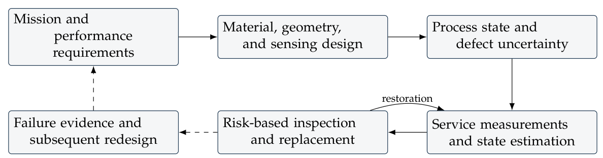
Failure analysis can feed subsequent designs by combining fracture-surface evidence, defect localization, interface inspection, and sensing records. Figure 1 distinguishes this proposed feedback from the implemented replacement loop. No fractography or physical root-cause experiment was performed. The benchmark records a specified crack-limit event; it cannot identify whether an actual fabricated component would fail by crack propagation, buckling, interface rupture, or another mechanism.
The design vector contains lattice relative density \(\rho^*\), shell thickness \(t_s\), route count \(n_s\), route width \(w_s\), orientation \(\theta\), finishing level \(z_p\), and inspection interval \(\tau_I\). The sampled trade-off vector is
A member is sample-nondominated if no other evaluated member improves at least one objective without worsening another. This finite-set definition does not imply global Pareto optimality in the continuous or mixed-variable design space.
The final admissibility conditions are
The first two are deterministic nominal checks, not probabilistic yield or displacement qualifications. Positive core dimensions and prescribed thickness/width ranges provide elementary geometric bounds, not manufacturing-process certification. \(P_{F,U}^{(1)}\) is an exact one-sided 95% upper binomial limit; \(A_L\) is the mean availability minus 1.96 Monte Carlo standard errors. The target reliability and availability values are illustrative design requirements and are not aerospace certification criteria.
With \(K\) structural failures in \(n\) independent lifecycles, \(\widehat P_F=K/n\). The binomial confidence construction follows Clopper and Pearson [16]; for \(K<n\),
where \(B^{-1}\) is the beta-distribution quantile. Two-sided 95% intervals use quantiles 0.025 and 0.975 with the usual endpoint conventions. A zero-failure run is reported with a finite upper probability bound, not as evidence of infinite physical reliability. The independent confirmation of the selected candidate avoids using its selection sample to make the final reliability statement; the bounds remain conditional on the assumed model and distributions.
For a realization with event times \(t_j\), the discounted cost is
Time in this equation is kh, 8.76 kh is one 365-day year, and \(r=0.04\) is annual. Costs are arbitrary consistent units, not quotations or industrial estimates. The outage integral is approximated on the simulation grid, while structural failure time is interpolated within the crossing step. Inspection, sensor repair, and replacement costs are charged only when their events occur. No separate unreported unscheduled-maintenance term is used: sensor repair is in \(C_S\), diagnostic loss in \(c_B\), and structural consequence in \(C_F\).
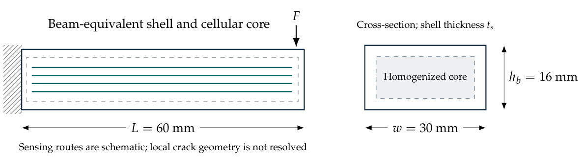
The notional bracket is a cantilever-equivalent member with length \(L=60\) mm and outer width and height \(w=30\) mm and \(h_b=16\) mm. It has a continuous shell and a homogenized cellular core. The example assumes a nominal metallic host with \(E_0=70\) GPa and density \(2700\,\mathrm{kg\,m^{-3}}\), together with separately integrated conductive sensing routes. No alloy, actual lattice topology, or process-specific metal–polymer interface is experimentally characterized. Figure 2 shows the modeling idealization, not a manufactured specimen or a finite-element mesh.
With \(w_i=w-2t_s\) and \(h_i=h_b-2t_s\), the response maps are
The density-squared stiffness contribution is an assumed bending-dominated homogenization inspired by cellular-solid scaling, for which Gibson and Ashby provide general background [17]. It is not a fitted property law for the unspecified core. The local nominal stress multiplier, displacement, and mass are
The last term is in kg with \(w_s\) in mm. Peak stress uses \(\Delta F=650\) N in the same map, while the fatigue range uses 300 N and service displacement uses 350 N. The fatigue-driving stress is held fixed as the crack progresses; local redistribution and crack-dependent stiffness are not solved. Its relationship to the normalized sensing damage term is prescribed rather than derived from a coupled finite-element model.
Table 2 specifies every random input governing unit life and sensing deterioration. Lognormal parameters are given as medians and standard deviations of the natural logarithm, avoiding ambiguity between arithmetic and logarithmic standard deviations. Defect and residual-stress truncation is implemented by inverse distribution functions. Unit variables are redrawn at replacement; persistent mission multipliers create dependence between successive units within a lifecycle even though primitive draws are independent.
| Input | Distribution | Persistence |
|---|---|---|
| Initial flaw \(a_0\) | Lognormal median \(75\,\mu\)m, log SD 0.45, truncated to 25–180 \(\mu\)m | Redrawn at unit replacement |
| Residual stress \(\sigma_r\) | Normal mean 120 MPa, SD 35 MPa, truncated to 40–220 MPa | Redrawn at unit replacement |
| Surface proximity \(\eta_s\) | Uniform \([0,1]\); larger is closer to surface | Redrawn at unit replacement |
| Morphology \(\chi\) | Uniform \([0,1]\) | Redrawn at unit replacement |
| Paris coefficient \(C\) | Lognormal median \(1.5\times10^{-11}\), log SD 0.35, units stated below Eq. (3) | Redrawn at unit replacement |
| Load multiplier \(\xi_L\) | Lognormal median 1, log SD 0.15 | Persistent over mission |
| Environment \(\xi_e\) | Lognormal median 1, log SD 0.15 | Persistent; affects growth and route outages |
| Drift multiplier \(\xi_b\) | Lognormal median 1, log SD 0.25 | Persistent over mission |
| Gain-aging multiplier \(\xi_f\) | Lognormal median 1, log SD 0.25 | Persistent over mission |
The remaining fixed maps are
Each missing route costs 12 units to repair at inspection. Functional refurbishment costs \(35+8n_s\). The structural-failure consequence is 500,000 units, diagnostic outage costs 60 units per kh, and \(\sigma_c=0.018\), \(\sigma_i=0.045\), \(\sigma_t=0.010\). These choices deliberately permit inspection and consequence costs to affect design ranking. They are scenario inputs, not universal engineering-economic parameters. Cost sensitivity to their magnitudes is an important application-specific task, not resolved by reporting precise Monte Carlo means.
The design set comprises 176 mixed-variable Latin-hypercube points generated with seed 61004 and four explicit reference members. The latter include a minimum-mass corner, the originally envisaged intermediate geometry, a high-reserve corner, and another intermediate reference. Every coordinate is supplied in design_candidates.csv; bounds appear in Table 3.
| Variable | Range | Type | Main modeled effect |
|---|---|---|---|
| \(\rho^*\) | 0.18–0.42 | Continuous | Core mass and stiffness |
| \(t_s\) | 1.2–2.8 mm | Continuous | Shell geometry |
| \(n_s\) | 1–4 | Integer | Route noise and availability |
| \(w_s\) | 0.5–1.4 mm | Continuous | Noise, aging, outage hazard |
| \(\theta\) | 0–90 degrees | Continuous | Prescribed stiffness/stress factors |
| \(z_p\) | 0 or 1 | Binary | Stress multiplier and finishing cost |
| \(\tau_I\) | 1–6 kh | Integer | Inspection and intervention timing |
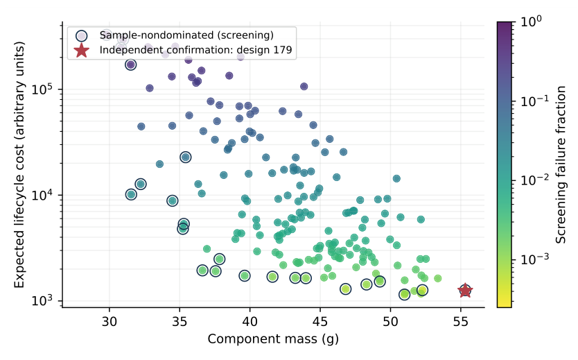
Each member is first simulated for 4,000 independent lifecycle realizations with a 0.25 kh time step and seed 1729. This is provisional screening rather than reliability certification. No member satisfies both confidence-based reliability and availability bounds in that screening run. Accordingly, uncertainty at the screening stage is not treated as proof that the design space is infeasible. Eight finalists are selected as the eight lowest estimated-cost designs satisfying nominal mechanical and diagnostic-availability checks. Each is independently evaluated using 50,000 realizations and seed \(40000+\mathrm{ID}\). The least-cost member satisfying all final constraints is selected; a fresh seed 92001 and 200,000 realizations provide its independent confirmation. All eight finalist results are included in the supplement, including those that do not qualify.
At each time step the code advances damage, gain loss, signed drift, and independent/common route events; checks structural-limit crossing before any inspection action; charges outage exposure only while the component remains structurally active; and performs scheduled inspection and repair when applicable. It then updates the estimator, predicts risk to the next inspection, and decides replacement. Inspections exactly at the mission endpoint are omitted. The simulation draws independent replacement-unit proposals for all trajectories at each inspection, making same-design policy comparisons reproducible with a shared random stream. Different route counts consume different random streams and are not treated as paired comparisons.
Table 4 reports representative finalist outcomes. Design 179 is the only finalist meeting both confidence-based lifecycle constraints in the refinement sample. Its parameters are \(\rho^*=0.42\), \(t_s=2.8\) mm, four routes, \(w_s=1.4\) mm, \(\theta=0\) degrees, finishing level one, and \(\tau_I=1\) kh. The independent confirmation gives mass 55.32 g, nominal displacement \(43.08\,\mu\)m, and nominal peak stress 61.61 MPa. Structural failure probability is 0.000455, the point reliability index is 3.317, and its one-sided lower bound is 3.268. Availability is 99.9673%, and mean cost is 1246.7 units with Monte Carlo standard error 23.1.
| ID | \(n\) | Mass (g) | \(10^3\widehat P_F\) | \(10^3 P_{F,U}^{(1)}\) | \(\beta_L^{(1)}\) | Cost (MCSE) |
|---|---|---|---|---|---|---|
| 27 | 50,000 | 50.99 | 1.080 | 1.355 | 2.999 | 1309.0 (71.1) |
| 169 | 50,000 | 52.17 | 2.200 | 2.577 | 2.797 | 1749.2 (100.5) |
| 174 | 50,000 | 48.29 | 1.080 | 1.355 | 2.999 | 1475.0 (71.1) |
| 180 | 50,000 | 46.80 | 1.360 | 1.664 | 2.936 | 1593.1 (79.6) |
| 179 | 200,000 | 55.32 | 0.455 | 0.542 | 3.268 | 1246.7 (23.1) |
The selected member lies on several upper design bounds. It is therefore a confidence-qualified result within the tested set, not evidence of an interior optimum or of the best possible AM bracket. Figure 3 shows the complete preliminary trade space and distinguishes its sample-nondominated points from independent confirmation. Low mass alone does not establish lifecycle admissibility. The minimum-mass corner passes the prescribed nominal displacement and stress checks but has a high simulated crack-limit exceedance probability; its economic comparison is not used to claim savings between equally admissible designs.
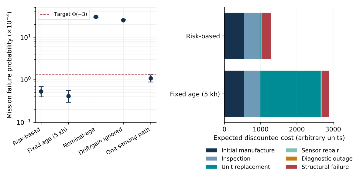
To separate policy effects from geometry effects, four maintenance rules are applied to the selected geometry. The risk rule uses Eq. (14). A fixed-age rule replaces at a specified unit age at scheduled inspections. Fixed ages from 2 to 20 kh are screened with 50,000 realizations each; 5 kh gives the lowest estimated cost among confidence-qualified ages on this integer grid. That policy is then compared independently with the risk rule using 100,000 realizations and seed 71001. The fixed-age search is not a proof of globally optimal age-based maintenance; its full results are supplied.
A nominal-age rule replaces when \(v_0t_{\mathrm{age}}\ge0.70\), ignoring the observed state for its replacement decision. A naive rule uses loaded measurements alone and assumes stable gain and drift. Both retain the same installed sensing hardware and inspection costs, so these are decision-policy ablations rather than sensor-removal experiments. A separate one-route design retains the mechanical geometry and route width but changes route count; it is assessed with an independent seed.
| Policy | Failures | \(10^3\widehat P_F\) | \(10^3 P_{F,U}^{(1)}\) | \(A\) (%) | Cost (MCSE) |
|---|---|---|---|---|---|
| Risk-based | 53 | 0.530 | 0.666 | 99.968 | 1283.7 (35.3) |
| Fixed age (5 kh) | 41 | 0.410 | 0.532 | 99.968 | 2880.0 (30.4) |
| Nominal-age | 3018 | 30.180 | 31.085 | 99.968 | 15099.6 (252.6) |
| Drift/gain ignored | 2509 | 25.090 | 25.919 | 99.968 | 12692.5 (230.3) |
| One sensing path | 108 | 1.080 | 1.267 | 98.025 | 1326.3 (49.9) |
Table 5 shows that risk-based replacement and the selected 5 kh fixed-age rule both satisfy the structural reliability target. Their point failure fractions differ slightly, but this comparison does not establish that the risk rule has lower structural failure probability. Its economic advantage comes primarily from avoiding scheduled replacements that are unnecessary for most realized fatigue rates. Expected cost falls by 55.4%, with an approximate paired delta-method 95% Monte Carlo interval of [53.1, 57.8]%. This interval concerns simulation sampling error under fixed assumptions, not uncertainty in industrial costs or the adequacy of the physical model.
The naive rule has markedly higher failure probability and damage-estimation error because gain loss can mask progression in its loaded-only signal. The nominal-age rule also fails to protect high-rate trajectories under the assumed latent distribution. Reducing the selected architecture to one route lowers diagnostic availability to approximately 98.03%, below the 99% requirement. This availability result should not be confused with a series-system failure probability. Figure 4 presents the structural intervals and the full cost decomposition for the two confidence-qualified same-geometry policies.
For the selected geometry at nominal uncertainty values, the integrated Paris life is \(8.89590864098\times10^6\) cycles. Independent numerical quadrature of the growth-law integral agrees to relative error \(4.19\times10^{-16}\). This verifies the analytical integration and its implementation, not the material validity of the assumed Paris coefficients. The observation matrix has rank three, and the reported total cost equals its stored component means to numerical rounding accuracy.
| \(n\) | Failures | \(10^3\widehat P_F\) | Two-sided 95% interval | \(\beta_L^{(1)}\) | Cost (MCSE) |
|---|---|---|---|---|---|
| 4,000 | 1 | 0.250 | [0.006, 1.392] | 3.039 | 1150.0 (121.7) |
| 20,000 | 8 | 0.400 | [0.173, 0.788] | 3.186 | 1221.1 (68.7) |
| 100,000 | 42 | 0.420 | [0.303, 0.568] | 3.267 | 1230.2 (31.3) |
| 200,000 | 91 | 0.455 | [0.366, 0.559] | 3.268 | 1246.7 (23.1) |
Table 6 and Figure 5 show why a small sample cannot provide a precise rare-failure statement. The 4,000-realization run observes only one failure, with a broad interval. The 200,000-realization confirmation observes 91, producing a narrower interval entirely below the target probability. This improvement is statistical precision conditional on the model. It does not remove systematic uncertainty in the fatigue or sensing assumptions.
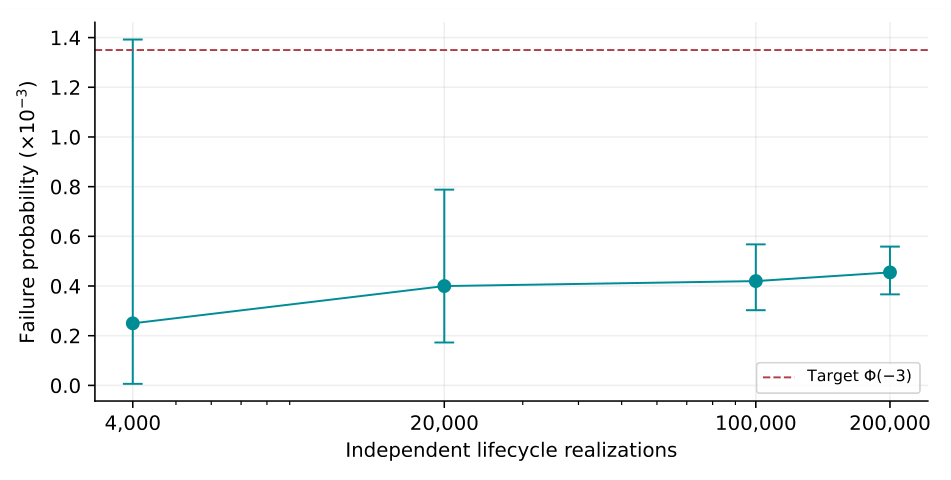
Table 7 compares 0.5, 0.25, and 0.125 kh steps. Failure-probability intervals overlap, and cost differences are comparable to Monte Carlo uncertainty. Availability changes by less than 0.01 percentage points over these runs. This is a limited refinement check: it supports the reported precision but does not establish asymptotic convergence for all possible parameter regimes. Inspections remain on integer-kilohour times, and structural crossing time is interpolated within the step.
| \(\Delta t\) (kh) | Failures | \(10^3\widehat P_F\) | Two-sided 95% interval | \(A\) (%) | Cost (MCSE) |
|---|---|---|---|---|---|
| 0.500 | 22 | 0.440 | [0.276, 0.666] | 99.9652 | 1238.5 (45.1) |
| 0.250 | 21 | 0.420 | [0.260, 0.642] | 99.9672 | 1229.5 (44.1) |
| 0.125 | 27 | 0.540 | [0.356, 0.786] | 99.9725 | 1288.3 (50.1) |
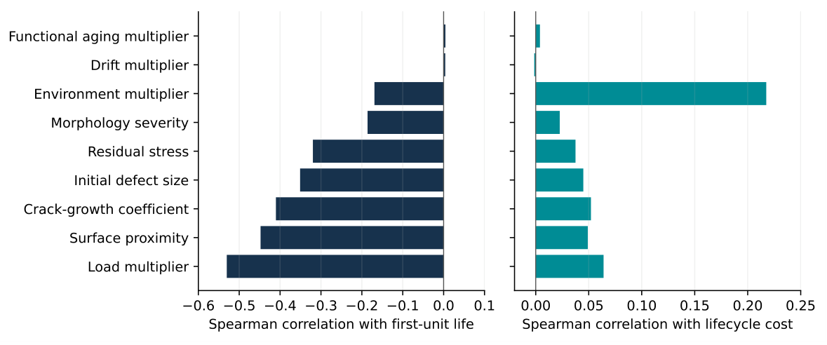
Spearman correlations are computed between the nine first-unit/persistent inputs and two outputs: intrinsic first-unit fatigue life without intervention, and full policy-dependent lifecycle cost. Figure 6 shows these signed associations. The strongest life association is load multiplier (\(-0.530\)), followed by surface proximity (\(-0.448\)), Paris coefficient (\(-0.410\)), initial defect size (\(-0.351\)), and residual stress (\(-0.320\)). The positive cost association is largest for environmental severity (\(0.218\)), which affects both fatigue and sensing-route outages.
These correlations are a screening description, not percentages of explained variance and not causal decompositions. Structural-unit variables are redrawn after replacement, so first-unit associations with lifecycle cost need not match their associations with unmaintained fatigue life. Sensor-aging and drift multipliers show near-zero marginal cost associations in this particular calibrated-interrogation scenario; this does not establish that they are negligible under different sensing or maintenance assumptions. Nominal elastic modulus is fixed and no modulus sensitivity ranking is claimed.
A useful physical sensing architecture should distinguish plausible mechanisms rather than merely flag a changed signal. Lack-of-fusion features, near-surface flaws, and roughness can motivate defect-sensitive fatigue investigations. Progressive conductive-network change can produce a persistent resistance offset, while temperature or electronics can generate reversible baseline shifts. Interface deterioration can reduce strain transfer and apparent gain. These mechanisms motivate unloaded, calibrated, and loaded interrogations, but the present linear response does not reproduce their material-specific electrical signatures.
A diagnostic feature set for experimental work could include irreversible baseline shift, load-correlated gain, hysteresis, temperature dependence, and disagreement between routes. A single-route change with stable mechanically equivalent routes would motivate examination of that route or interface. A correlated change across every route would require checking shared thermal/electronic disturbances as well as structural damage. Reduced gain with a stable unloaded baseline would motivate a strain-transfer assessment. These are testable diagnostic hypotheses, not uniquely validated classification rules.
The common-cause hazard deliberately prevents route count from being treated as unlimited protection. Calibration and local repair restore information at inspection, but diagnostic outages between inspections remain in the availability and cost records. Translating this mechanism to a real component requires a measured probability of detection, false-alarm behavior, calibration uncertainty, and route-dependence model. No confusion matrix or classification accuracy is reported because no mechanism-labeled experimental dataset was obtained.
The nominal response maps favor thinner shells and lower core density through reduced mass. The fatigue model instead amplifies adverse combinations of stress, defects, morphology, and residual stress. A candidate can satisfy the deterministic stress/displacement checks while failing the mission probability requirement. Confidence-based screening also reveals a different limitation: at low sample sizes, uncertainty in a rare failure estimate can prevent a reliability claim even when a subsequent independent evaluation qualifies the design.
The selected corner combines mechanical reserve, four sensing routes, wide tracks, finishing, and frequent inspection. Its location on multiple bounds indicates that the tested ranges constrain the apparent optimum. A wider design domain, other topologies, or a different consequence cost could change the selected member. The finite sample and finalist shortlist do not prove that no lower-cost qualifying design exists elsewhere. Increasing structural reserve has a material cost, but the objective is expected mission performance rather than minimum initial mass.
The same-geometry comparisons show that a reliable monitoring model changes intervention frequency. The fixed-age rule replaces nearly three units per mission even though the selected bracket’s nominal unmaintained fatigue life is approximately 89 kh. Risk-based replacement is infrequent for nominal trajectories but can respond to adverse rates inferred from inspections. The gain/drift-aware contrast is central: a loaded-only decision rule can incorrectly interpret a reduced functional response as low structural damage.
The cost benefit is conditional on the assumed failure consequence, inspection access, and possibility of rapidly repairing sensing routes. Changing these assumptions could reverse the preferred architecture or policy. The example does not establish that four routes and a one-kilohour interval are optimal for actual hardware. Nor does it establish that state-based maintenance always reduces failure probability relative to a conservative age policy. In the verified comparison, both confidence-qualified policies meet the same illustrative structural target, while their lifecycle costs differ substantially.
Physical qualification should preserve the material–process–geometry and sensor–host interactions represented in service. Static coupons alone would not identify crack progression, calibration aging, or route-dependence behavior. Defect characterization, surface metrology, interface tests, environmental exposure, and blind detection trials supply different types of evidence. The benchmark’s separation of structural reliability and diagnostic availability makes their acceptance requirements explicit rather than combining them into an unexplained scalar score.
The dominant rank associations are also model-dependent. Cubic stress dependence is prescribed by the Paris exponent, and the environment input intentionally influences both fatigue and route outage. Their observed rankings partly reflect these modeling choices. Reliability statements must therefore be accompanied by distribution provenance and model-form checks when the framework is applied to a specific material system.
A transparent lifecycle framework has been developed for a AM self-sensing structure. The model distinguishes structural progression, functional gain loss, and signed measurement drift; gives redundancy a finite, noise- and outage-based interpretation; and connects sequential damage estimation to a stated replacement rule. Manufacturing, inspection, replacement, sensing repair, diagnostic outage, and structural consequence appear explicitly in the cost accounting.
The independently confirmed selected design satisfies the benchmark’s confidence-based structural and diagnostic criteria, with 91 structural-limit exceedances in 200,000 lifecycles and a one-sided reliability-index lower bound of 3.268. Same-geometry comparisons show 55.4% lower expected cost than the least-cost qualified fixed-age policy identified on the tested integer-age grid. Both policies meet the illustrative structural requirement; the evidence supports an economic difference rather than a universal reliability advantage of condition-based maintenance. Loaded-only monitoring and nominal-age replacement are inadequate under the assumed latent variability, while a one-route architecture fails the separate diagnostic-availability requirement.
The results are newly executed computations with complete parameter, code, and output provenance. Their contribution is an explicit treatment of information quality in a lifecycle decision model. Material-specific fatigue, sensing, interface, process, and economic calibration remains necessary before industrial interpretation or qualification.
This research received no external funding.
The author declares that there are no competing interests.
The data supporting the findings of this study are available from the author upon reasonable request.
Generative artificial intelligence tools were used solely for language editing, grammatical correction, and improvement of readability. The author reviewed and verified the final manuscript and assumes full responsibility for its accuracy, integrity, and scholarly content.