
Collaborative robotic motion requires coordinated treatment of task execution and physical interaction. ISO 10218-1:2025 addresses safety requirements for industrial robots and provides the robot-level context for control implementation [1]. ISO 10218-2:2025 addresses industrial robot applications and cells, extending the engineering scope to integration and application-level hazards [2]. ISO/TS 15066 supplies guidance specifically concerned with collaborative industrial robot systems [3]. ISO/PAS 5672 describes measurement and analysis of contact forces and pressures, including the characteristics of pressure-force measurement devices [4]. These documents motivate careful physical evaluation, but a controller simulation does not establish conformity with their requirements.
Impedance control represents interaction through a desired mechanical response. Hogan’s foundational formulation explains why motion and force regulation must be considered together when a manipulator is mechanically coupled to its environment [5]. Khatib’s operational-space formulation provides a task-coordinate framework for manipulator motion and force control [6]. The present investigation uses a scalar local model to make actuator work and controller switching transparent. It does not equate that model with a complete manipulator.
An important implementation distinction arises when a supervisor reduces automation authority. Multiplying an entire impedance expression by a small coefficient reduces both reference-driving action and velocity-opposing feedback. Under externally applied force, the loss of damping can increase motion even when commanded task authority decreases. A second distinction concerns finite energy reserves. Evaluating actuator power only at the start of an interval can miss work generated as an applied force accelerates a stationary body. These two issues are investigated separately before their interaction is assessed.
Kronander and Billard examine stability considerations for variable impedance and demonstrate the importance of the way impedance parameters evolve [7]. Their work motivates explicit treatment of gain changes rather than an assumption that positive instantaneous gains establish closed-loop stability.
Ferraguti, Secchi, and Fantuzzi use an energy tank to regulate variable-stiffness impedance control [8]. The present study builds on the broader idea of accounting for mechanically exchanged energy. Its reserve is a virtual actuator-work account, and its analysis is stated for a scalar held-force model.
Michel, Ott, and Lee combine hierarchical variable compliance, redundancy, energy tanks, and a safety layer [9]. This establishes that energy-aware compliance coordination is existing work. The present manuscript does not claim to originate that combination.
Jadav and colleagues already combine interaction-dependent autonomy allocation, variable impedance, and energy-tank-based task passivation [10]. Consequently, interaction-responsive authority is not treated here as an unexplored research gap. The distinction investigated in this manuscript is how authority enters the dissipative feedback and how the final saturated force is constrained by a within-interval work budget.
Michel, Saveriano, and Lee formulate energy tanks using control barrier functions to enforce energy and power constraints [11]. Their continuous tank construction and robot experiments address a broader control problem. The present gate instead uses a scalar comparison envelope, a closed-form branch, and a bracketed search branch to constrain the work associated with a held force.
Benzi, Ferraguti, and Secchi examine energy-tank control for constraints motivated by ISO/TS 15066 [12]. Their approach emphasizes the difference between energy limits and conservative velocity constraints. Here, the numerical comparisons additionally expose circumstances in which maintaining an actuator-work reserve does not reduce externally induced peak speed.
Tian and colleagues extend energy-aware impedance to safety null-space compliance in redundant robots [13]. That contribution underscores the additional energy channels encountered in multi-axis systems; these channels remain outside the scalar analysis developed below.
The contribution is therefore a reduced-order implementation study with three concrete elements: a damping-preserving authority law; a sign-aware, saturation-aware interval-work gate with a conditional reserve guarantee; and an executable comparison that separates supervisory shaping, reserve enforcement, and their limitations. No claim of exhaustive priority over all energy-tank formulations is made. The value of the study lies in its explicit equations, diagnostic counterexamples, and reproducible evidence.
The local translational plant is
where \(x\) is position, \(v\) is velocity, \(m>0\) is effective mass, \(b\geq0\) is viscous dissipation, \(u\) is the applied actuator force, and \(f_h\) is an external force. Actuation is constant during each interval \([t_k,t_{k+1})\) of length \(h_k\). The simulated external input is also held at its interval-start sample; the gate’s comparison argument only requires a bounded external input and does not require it to be constant.
The reference is \((x_r,v_r)\), with \(v_r=\dot x_r\). Measured velocity is denoted \(\hat v_k\) and the force signal used for supervisory shaping is \(\hat f_{h,k}\). The gate assumes
These are explicit model assumptions. The force limit \(F_H\) bounds the physical external input; it is not the risk normalization \(F_s\), an actuator limit, or a biomechanical threshold.
The supervisory index is
where \(F_s,V_s>0\) and \(\beta\geq0\). This index is a dimensionless scheduling variable. It is not an estimated probability of injury or a validated clinical or industrial risk score. Its weights are design choices examined through sensitivity tests.
With \(0\leq\alpha\leq1\), \(K_{\max}\geq K_{\min}>0\), \(D_0>0\), and nonnegative \(\Delta D,B_r\), the scheduled stiffness, damping, and reference authority are
The requested force is
Thus the reference-driving terms are reduced by \(a_k\), while velocity-opposing damping remains outside that multiplier. The additional term \(B_r r_k\hat v_k\) increases interaction braking. This algebraic separation is the central difference from the diagnostic coupled-authority controller.
Physical force clipping occurs before budget gating:
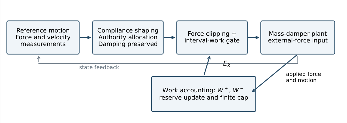
Budget calculations concern the final applied force \(u_k\), rather than the unsaturated request. Figure 1 shows the implemented information flow. A production task executive could supply the reference and mode settings; no discrete manufacturing task automaton or contact estimator is implemented in this study.
For a held actuator force, positive and negative mechanical work are defined separately:
Here \([z]_+=\max(z,0)\). The distinction prevents positive and negative work within an interval from cancelling in the debit. The available positive-work budget is
The reserve \(E_k\) is virtual mechanical-work bookkeeping. It does not represent measured electrical battery charge or experimentally established regeneration efficiency.
Let a candidate applied force have amplitude \(R=|u_k|\) and direction \(s=\operatorname{sign}(u_{c,k})\). An upper bound on initial directional velocity is
When directional velocity is nonnegative, its growth is at most \((R+F_H)/m_\ell\), because viscous damping cannot accelerate it in the force direction. If initial directional velocity is negative, an upper comparison dynamics uses \(b_u\) and \(m_\ell\) until it reaches zero. For \(b_u>0\), the earliest comparison crossing is
Before this time the comparison velocity is negative and therefore cannot contribute positive actuator work. After the crossing, ignoring viscous damping gives a conservative positive-velocity envelope. Integrating that envelope yields
Set \(\mathcal H(0,y,h)=0\). Under Eq. (2), \(W_k^+\leq\mathcal H(R,y_k,h_k)\). The negative-velocity branch is important: a force that remains dissipative throughout the interval is admitted without a positive-work debit. A velocity-independent acceleration bound would unnecessarily suppress such braking near reserve depletion.
Write \(R_c=|u_{c,k}|\). If \(\mathcal H(R_c,y_k,h_k)\leq C_k\), select \(\gamma_k=1\). Otherwise select the largest feasible fraction satisfying
For \(y_k\geq0\), define
The feasible root is evaluated using a numerically stable expression:
When \(C_k=0\) and the full force is infeasible, this branch gives \(\gamma_k=0\). A zero force request gives \(\gamma_k=1\) with zero work. For \(y_k<0\), the envelope is nondecreasing with amplitude: \(R(R+F_H)\) increases and the crossing time decreases as \(R\) increases. A 48-iteration bisection retains a feasible lower endpoint and returns that endpoint. This branch can admit nonzero dissipative forces even when \(C_k=0\).
The account is updated after the interval:
Negative actuator work replenishes a fraction \(\eta\) of the virtual reserve. Plant viscous loss is not also credited, avoiding a second credit for the same energy path. There is no lower clipping: the gate must enforce the lower bound before work is released. Define discarded reserve at the cap as \(L_k=\left[\widetilde E_{k+1}-E_{\max}\right]_+\).
Proposition 1 (Reserve invariance and sampled port-energy inequality). Suppose Eq. (2) holds, applied force is held during each interval, \(E_0\in[E_{\min},E_{\max}]\), and signed work is accounted for exactly. Then the gate and ledger maintain \(E_k\in[E_{\min},E_{\max}]\). With physical kinetic energy \(T_k=mv_k^2/2\) and storage \(S_k=T_k+E_k-E_{\min}\),
where \(W_{h,k}=\int f_hv\,\mathrm dt\) and \(Q_k=\int bv^2\,\mathrm dt\geq0\) over the interval.
Proof. In directional coordinates \(z=sv\), for \(z<0\) the plant derivative is bounded above by \((R+F_H-b_uz)/m_\ell\). For \(z\geq0\) it is bounded above by \((R+F_H)/m_\ell\). Starting the comparison at \(y_k\geq z_k\) gives Eq. (11). The gate therefore ensures \(W_k^+\leq C_k\). Eq. (15) implies \(\widetilde E_{k+1}\geq E_{\min}\); applying the upper cap preserves this lower bound and establishes invariance by induction. Integrating the physical power balance gives \(T_{k+1}-T_k=W_k^+-W_k^-+W_{h,k}-Q_k\). Adding the reserve change gives Eq. (16). \(\square\)
Two useful cumulative consequences are
and
The latter is not an absolute human-interaction kinetic-energy limit: external work can increase the right-hand side. The sampled inequality also does not prove asymptotic tracking, multi-axis robot stability, or safety certification. Exact accounting is an explicit assumption; unbounded force, underestimated mass bounds, unknown velocity error, or inaccurate work integration can invalidate the guarantee.
The supplied implementation regenerates the state histories and performance metrics from the equations and parameters below.
The nominal reference is
with its analytic derivative used as \(v_r(t)\). The external input is
The horizon is 8 s, with \(h=1\) ms and initial conditions \(x_0=v_0=0\). Nominal force and velocity measurements are exact. Table 1 gives every controller and gate constant used in the main experiments. The well-funded reserve is \(E_0=3\) J; a second experiment uses \(E_0=0.1\) J without changing any physical or supervisory parameter.
| Symbol | Value | Unit | Role |
|---|---|---|---|
| \(m\), \(b\) | 2.2, 6 | kg, Ns/m | Actual simulated mass and viscous dissipation |
| \(K_{\min}\), \(K_{\max}\) | 180, 600 | N/m | Scheduled stiffness range |
| \(D_0\), \(\Delta D\) | 48, 40 | Ns/m | Base damping and interaction increment |
| \(B_r\) | 12 | Ns/m | Additional interaction braking |
| \(F_s\), \(V_s\) | 40, 0.5 | N, m/s | Heuristic force and speed normalizations |
| \(\beta\), \(\alpha\) | 0.2, 0.65 | – | Speed contribution and authority reduction |
| \(U_{\max}\) | 95 | N | Applied-force saturation magnitude |
| \(E_{\min}\), \(E_{\max}\) | 0.05, 6 | J | Reserve lower bound and upper cap |
| \(E_0\), \(\eta\) | 3 or 0.1, 0.6 | J, – | Initial reserve and negative-work credit fraction |
| \(m_\ell\), \(b_u\) | 1.5, 12 | kg, Ns/m | Bounds used by the comparison envelope |
| \(F_H\) | 90 | N | Bound on actual external-force magnitude |
| \(\varepsilon_v\) | 0 | m/s | Nominal velocity-error bound |
For positive \(b\), let \(\lambda=b/m\), \(w_k=(u_k+f_{h,k})/b\), and \(c_k=(1-e^{-\lambda h})/\lambda\). On a held-input interval,
and the exact state update is
Velocity is monotone on each interval and can cross zero at most once. If a crossing occurs, the code splits the actuator-work integral at that crossing before calculating \(W^+\) and \(W^-\). Viscous loss and external work are integrated analytically as well. This permits a direct check of the physical energy balance independently of reserve bookkeeping.
The update order is: sample reference and measurements; compute \(r,K,D,a\); request force; clip force; evaluate the budget gate; propagate the plant and integrate work; update and cap the reserve; advance time. Work is always calculated from the applied force. All gain changes occur at interval boundaries. No hidden force filter, numerical differentiation, or task-state switch is used.
Table 2 defines eight configurations. The matched fixed controller uses the same zero-risk stiffness and damping as the proposed controller. The conservative fixed controller provides a simple low-stiffness, high-damping comparator. Component tests are numerical configurations, not implementations of the cited literature methods; no performance superiority over those published methods is claimed.
For controllers without a gate, the same work-account equation is evaluated only as a diagnostic shadow account. It does not influence their forces and may fall below \(E_{\min}\) or zero. Such a negative diagnostic value means that the corresponding force history would violate the selected budget; it does not imply a physical negative battery charge.
| Code | Configuration | Force request before clipping |
|---|---|---|
| F | Matched fixed impedance | \(K_{\max}(x_r-x)+D_0(v_r-\hat v)\) |
| C | Conservative fixed impedance | \(K_{\min}(x_r-x)+(D_0+\Delta D)(v_r-\hat v)\) |
| V | Compliance only | \(K_k(x_r-x)+D_k(v_r-\hat v)\) |
| A | Authority only | \(a_k[K_{\max}(x_r-x)+D_0v_r]-D_0\hat v\) |
| CA | Coupled authority diagnostic | \(a_k[K_k(x_r-x)+D_k(v_r-\hat v)]-B_rr_k\hat v\) |
| S | Supervisor without gate | Eq. (5), with \(\gamma=1\) |
| G | Work gate only | F force request, followed by Eqs. (6)–(12) |
| SG | Complete controller | S force request, followed by the same gate |
The deterministic grid comprises \(m\in\{1.6,2.2,2.8\}\) kg, \(b\in\{3,6,9\}\) Ns/m, and force multipliers \(q_f\in\{0.6,1.0,1.4\}\), giving 27 configurations. F, C, CA, S, and SG are evaluated with a 3 J initial account; SG is additionally evaluated with a 0.1 J reserve in every grid configuration.
Fifty paired scenarios are generated with a fixed seed, 20261005. Mass is uniform on \([1.6,2.8]\) kg, dissipation on \([3,9]\) Ns/m, force multiplier on \([0.6,1.4]\), and reference-amplitude multiplier on \([0.75,1.25]\). The low-frequency reference phase is uniform on \([-0.5,0.5]\) rad. Force-measurement delay is selected with equal probability from 0, 5, and 15 ms. At each interval, independent force noise is uniform on \([-2,2]\) N and velocity noise is uniform on \([-0.02,0.02]\) m/s. The gate uses \(\varepsilon_v=0.025\) m/s. Actual external forces remain below 81.2 N, within \(F_H=90\) N.
Each configuration receives the same scenario parameters and the same measurement-noise realization, with seed \(1000+i\) for scenario \(i\). Both reserve levels are tested for all eight controllers. Force delay affects scheduling through \(r\); the budget envelope uses the independently specified physical force bound rather than the delayed force signal. The actual plant parameters are used for exact work evaluation in the simulator. Therefore these scenarios test the gate’s coarse-bound construction, not an uncertain hardware work estimator.
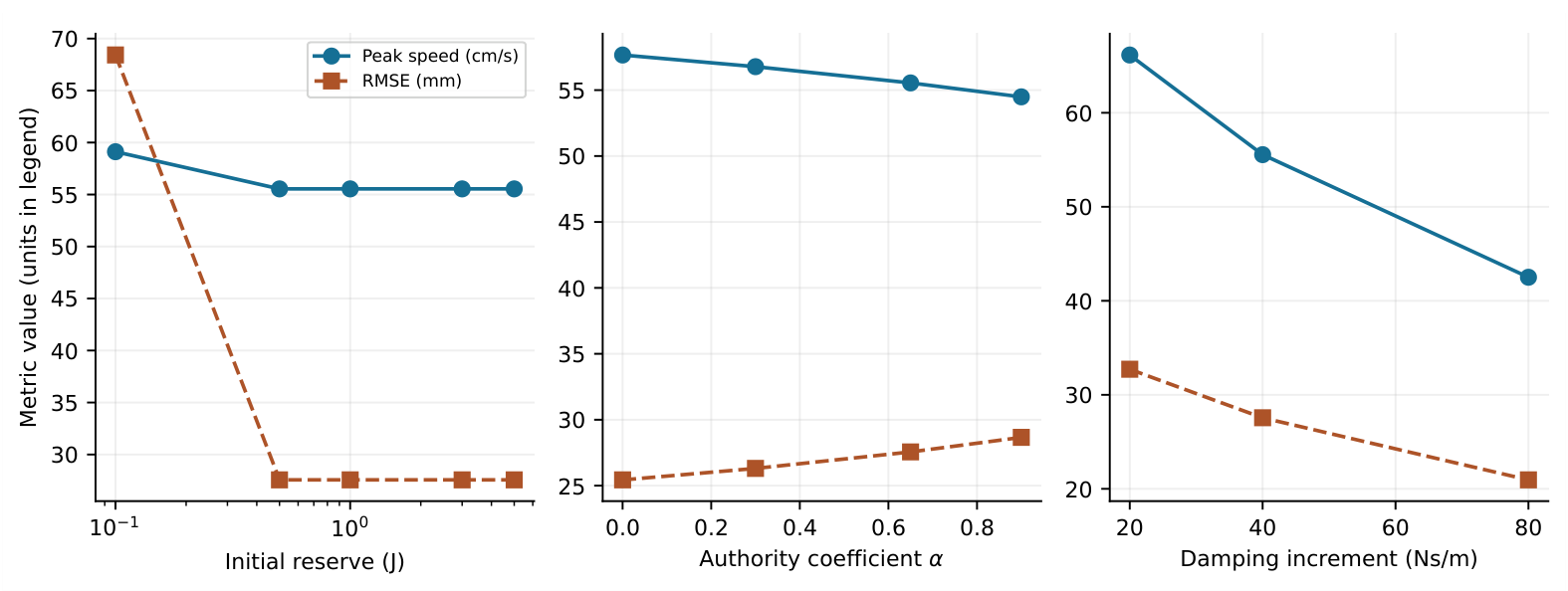
One-at-a-time sensitivity tests vary \(E_0\in\{0.1,0.5,1,3,5\}\) J, \(\alpha\in\{0,0.3,0.65,0.9\}\), \(F_s\in\{20,40,80\}\) N, \(\Delta D\in\{20,40,80\}\) Ns/m, and \(F_H\in\{82,90,120\}\) N. Other values remain nominal. These are descriptive design sweeps, not an optimization procedure or a global parameter-importance analysis.
Tracking error is evaluated at interval starts:
Peak speed is the maximum of interval-endpoint absolute velocities, which is also the continuous interval maximum because velocity is monotone within each held-input interval. Peak kinetic energy is \(m v_{\mathrm{peak}}^2/2\) for each constant-mass run. Positive and negative actuator work, external work, viscous loss, minimum reserve, cap spillage, and the fraction of intervals with \(\gamma<1-10^{-10}\) are also exported. Event-specific speed and RMSE metrics are supplied in the data package.
The code checks force saturation, physical energy-balance residuals, reserve invariance, interval-work envelope compliance, and Eq. (17). Four hundred independent random held-input cases compare analytic positive work with adaptive numerical quadrature, including intervals with velocity reversal. A separate at-rest diagnostic tests the inadequacy of an interval-start power calculation. Finally, steps of 2, 1, 0.5, and 0.25 ms are compared at both reserve levels. Because the plant update is exact for held inputs, this last comparison measures changes in the sampled policy and force approximation, rather than errors from a plant integration algorithm.
Table 3 reports the nominal component comparison. SG reduces peak speed by 10.85% and peak kinetic energy by 20.52% relative to F, with a 42.08% increase in tracking RMSE. These results are a specific trade-off under the selected reference and force history. The proportional kinetic-energy reduction follows directly from the speed reduction at fixed mass and is not an independent statistical outcome.
| Controller | RMSE (mm) | Peak speed (cm/s) | Peak \(T\) (J) | \(\sum W^+\) (J) | Gate (%) |
|---|---|---|---|---|---|
| F | 19.40 | 62.31 | 0.427 | 1.784 | 0.00 |
| C | 40.68 | 64.39 | 0.456 | 0.994 | 0.00 |
| V | 28.08 | 63.62 | 0.445 | 1.931 | 0.00 |
| A | 31.88 | 81.91 | 0.738 | 2.706 | 0.00 |
| CA | 54.96 | 109.63 | 1.322 | 3.663 | 0.00 |
| S | 27.56 | 55.55 | 0.339 | 1.589 | 0.00 |
| G | 19.40 | 62.31 | 0.427 | 1.784 | 0.00 |
| SG | 27.56 | 55.55 | 0.339 | 1.589 | 0.00 |
The reserve gate does not activate at \(E_0=3\) J. Consequently, the nominal speed reduction cannot be attributed to energy-budget enforcement: it arises from the damping-preserving supervisory law. This distinction is directly visible in the equality of F with G and of S with SG. Reporting this inactive-gate regime prevents a gain-scheduling effect from being presented as evidence for the budget mechanism.
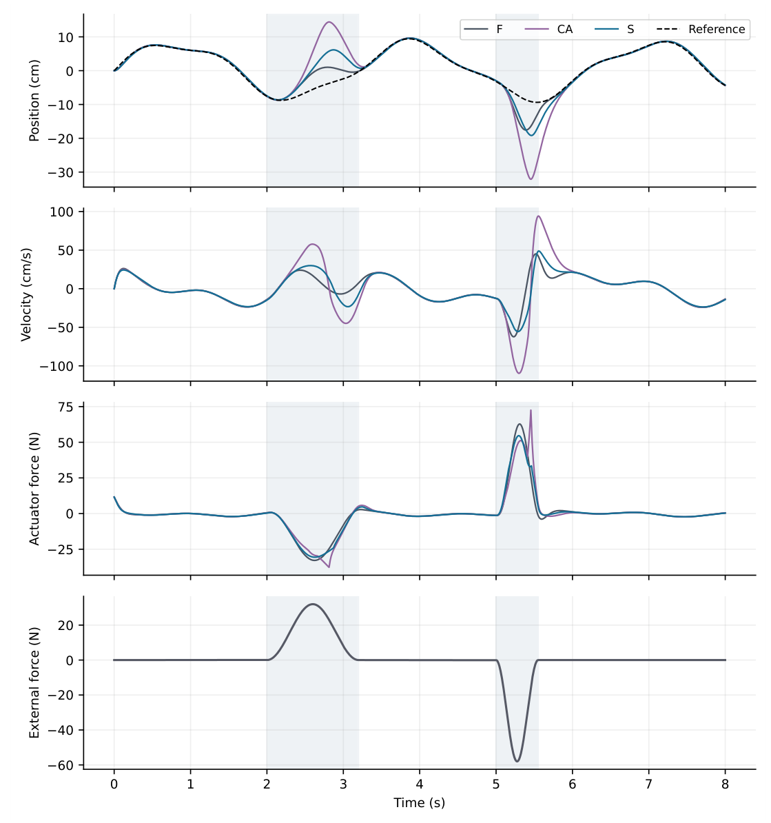
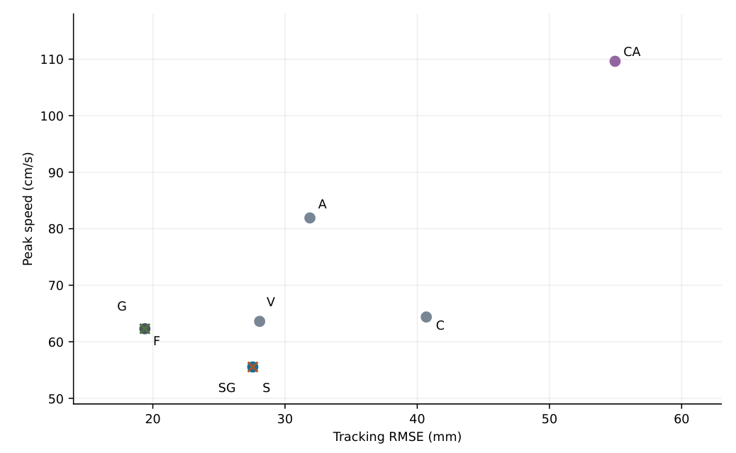
The coupled-authority diagnostic CA reaches a peak speed of 109.63 cm/s, exceeding both F and S. V and C also fail to reduce peak speed in this nominal test, while A increases it. Figure 2 shows the corresponding dynamics. Figure 3 places the component configurations in the tracking-error versus peak-speed plane. These comparisons establish the importance of preserving damping for this particular implementation, rather than a general theorem that softer or more autonomous controllers are safer.
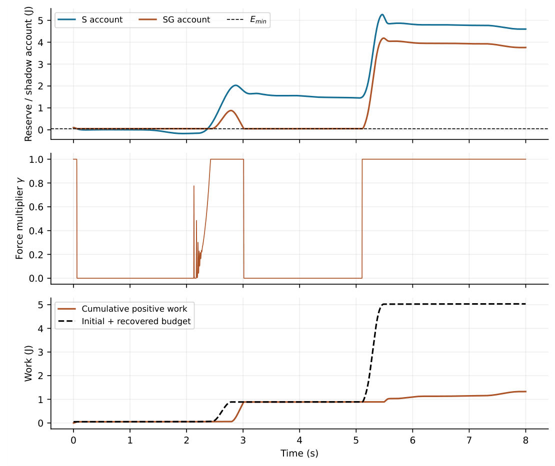
The 0.1 J experiment activates the budget constraint. Table 4 distinguishes controlled reserves from unconstrained shadow accounts. F and S have shadow-account minima below zero, so their force histories do not satisfy the selected resource constraint. SG maintains the 0.05 J reserve lower bound and activates its gate during 55.76% of intervals. Its RMSE increases to 68.42 mm and peak speed is 59.12 cm/s.
| Controller | RMSE (mm) | Peak speed (cm/s) | \(\sum W^+\) (J) | Min. account (J) | Gate (%) |
|---|---|---|---|---|---|
| F | 19.40 | 62.31 | 1.784 | -0.179 | 0.00 |
| S | 27.56 | 55.55 | 1.589 | -0.170 | 0.00 |
| G | 70.18 | 146.24 | 1.151 | 0.050 | 64.06 |
| SG | 68.42 | 59.12 | 1.328 | 0.050 | 55.76 |
G maintains the reserve but reaches a peak speed of approximately 146.24 cm/s, substantially exceeding F. This is an important counterexample: constraining positive actuator work can weaken task-restoring action while external forcing continues to inject energy. SG’s preserved damping improves its response relative to G in this case, but does not eliminate the tracking penalty of a depleted reserve. Figure 4 shows the reserve, gate activity, and cumulative work budget. Lower-bound compliance is achieved without resetting a negative reserve to the permitted range.
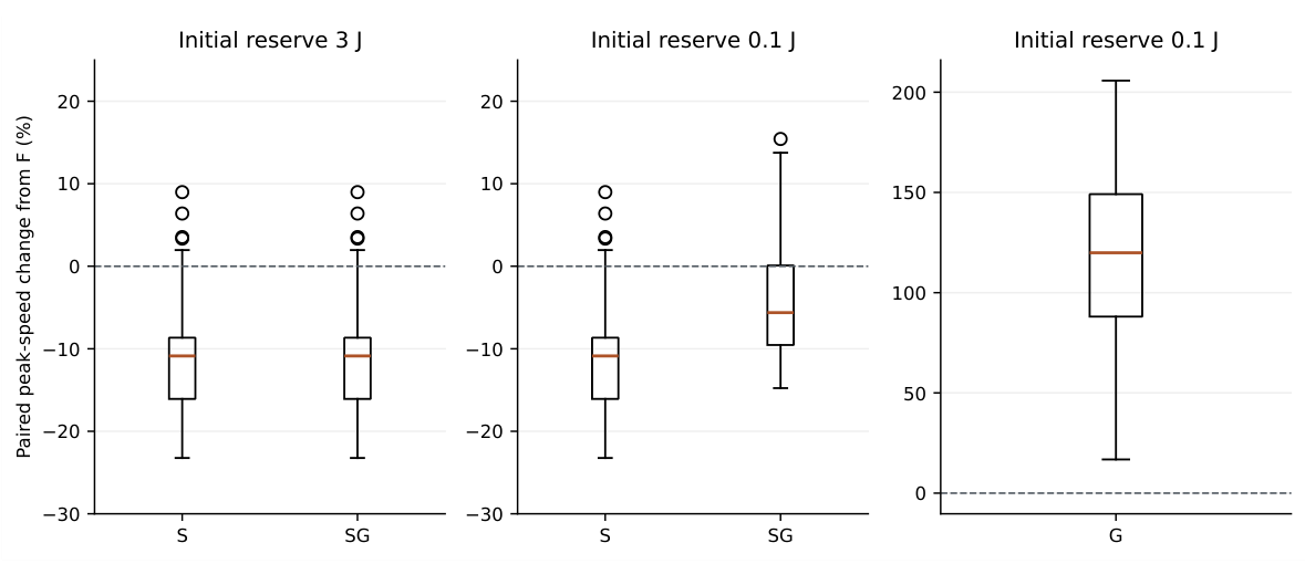
Within the 27-configuration deterministic grid, SG reduces nominal peak speed relative to F in every configuration; reductions range from 3.94% to 20.46%. The paired perturbation ensemble gives a more qualified result. At the 3 J reserve, SG reduces peak speed in 45 of 50 cases, with a median paired change of \(-10.87\%\) and a range from \(-23.24\%\) to \(+8.99\%\). At the 0.1 J reserve, it reduces peak speed in 37 of 50 cases, with a median change of \(-5.62\%\) and a range from \(-14.77\%\) to \(+15.43\%\).
Table 5 and Figure 5 show that the median effect does not establish a universal speed benefit. The SG reserve remains at or above 0.05 J throughout every low-reserve perturbation run, while its median tracking RMSE is approximately 64.43 mm. Hardware
or population-level conclusions cannot be drawn from these scenario distributions. They are intended to expose controller sensitivity and reproduce the exceptions to the nominal trend.
| \(E_0\) (J) | Controller | RMSE median [IQR] (mm) | Speed median [IQR] (cm/s) | Gate median (%) |
|---|---|---|---|---|
| 3.0 | F | 18.37 [15.51, 21.28] | 61.69 [53.59, 66.86] | 0.00 |
| 3.0 | S | 26.31 [20.48, 32.97] | 54.02 [46.32, 60.62] | 0.00 |
| 3.0 | G | 18.37 [15.51, 21.28] | 61.69 [53.59, 66.86] | 0.00 |
| 3.0 | SG | 26.31 [20.48, 32.97] | 54.02 [46.32, 60.62] | 0.00 |
| 0.1 | F | 18.37 [15.51, 21.28] | 61.69 [53.59, 66.86] | 0.00 |
| 0.1 | S | 26.31 [20.48, 32.97] | 54.02 [46.32, 60.62] | 0.00 |
| 0.1 | G | 62.53 [54.31, 70.06] | 129.99 [121.55, 141.51] | 63.68 |
| 0.1 | SG | 64.43 [58.13, 72.72] | 56.35 [51.87, 63.53] | 47.86 |
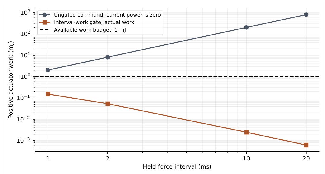
At rest, a current-power calculation gives \(u_kv_k=0\) for any force request, although held force subsequently accelerates the plant. With \(u_c=95\) N, \(f_h=0\), \(v_0=0\), and an available budget of 1 mJ, an unmodified force command releases approximately 2.049 mJ during a 1 ms interval. It therefore violates that budget even at the nominal update rate. Table 6 reports four interval lengths. The interval-work gate enforces the available budget in every diagnostic case; Figure 6 shows the separation between actual gated work and ungated work.
| \(h\) (ms) | \(W^+_{\mathrm{current}}\) (mJ) | \(\gamma\) | \(W^+_{\mathrm{gated}}\) (mJ) | Gated \(E_1\) (J) |
|---|---|---|---|---|
| 1 | 2.049 | 0.272497 | 0.152168 | 0.050848 |
| 2 | 8.190 | 0.080824 | 0.053499 | 0.050947 |
| 10 | 203.262 | 0.003496 | 0.002484 | 0.050998 |
| 20 | 805.738 | 0.000876 | 0.000619 | 0.050999 |
Step refinement produces stable well-funded metrics (Table 7). From 1 to 0.25 ms, F’s RMSE changes by approximately 0.029% and peak speed by 0.120%; SG’s RMSE changes by approximately 0.017% and peak speed by 0.045%. Low-reserve operation has stronger sampling dependence: SG’s RMSE decreases from 68.42 mm at 1 ms to 58.20 mm at 0.25 ms, while gate activity decreases from 55.76% to 39.85%. Peak speed changes from 59.12 to 58.92 cm/s and reserve invariance is retained. The larger tracking change reflects a different sampled budget policy and its interaction with trajectory lag. Consequently, the low-reserve 1 ms results describe that specific update rate; they are not claimed to be independent of sampling period.
| \(E_0\) (J) | Step (ms) | Controller | RMSE (mm) | Peak speed (cm/s) | Gate (%) |
|---|---|---|---|---|---|
| 3.0 | 2.00 | F | 19.405 | 62.409 | 0.00 |
| 3.0 | 2.00 | SG | 27.566 | 55.581 | 0.00 |
| 3.0 | 1.00 | F | 19.397 | 62.308 | 0.00 |
| 3.0 | 1.00 | SG | 27.560 | 55.547 | 0.00 |
| 3.0 | 0.50 | F | 19.394 | 62.258 | 0.00 |
| 3.0 | 0.50 | SG | 27.557 | 55.531 | 0.00 |
| 3.0 | 0.25 | F | 19.392 | 62.234 | 0.00 |
| 3.0 | 0.25 | SG | 27.555 | 55.522 | 0.00 |
| 0.1 | 2.00 | F | 19.405 | 62.409 | 0.00 |
| 0.1 | 2.00 | SG | 69.736 | 60.203 | 56.00 |
| 0.1 | 1.00 | F | 19.397 | 62.308 | 0.00 |
| 0.1 | 1.00 | SG | 68.422 | 59.120 | 55.76 |
| 0.1 | 0.50 | F | 19.394 | 62.258 | 0.00 |
| 0.1 | 0.50 | SG | 58.718 | 59.296 | 40.23 |
| 0.1 | 0.25 | F | 19.392 | 62.234 | 0.00 |
| 0.1 | 0.25 | SG | 58.200 | 58.918 | 39.85 |
The 400 random work-integration checks have a maximum discrepancy from adaptive quadrature of approximately \(1.25\times10^{-14}\) J. Every simulated gated interval satisfies the comparison envelope within the specified numerical tolerance, and every run satisfies the physical energy-balance and force-saturation checks. The complete residuals and assertion thresholds are supplied with the code rather than inferred from rounded table entries.
Figure 7 illustrates selected one-at-a-time sweeps. A larger initial reserve reduces or removes budget-induced tracking restrictions. Changing authority reduction and damping increment also changes externally driven motion; their effects should be examined jointly before application-level tuning. The complete \(F_s\) and \(F_H\) sweeps are provided as CSV data. These finite sweeps characterize the specified design choices; they do not identify globally optimal gains, and no optimization-based tuning procedure is claimed.
The experiments separate three mechanisms that can otherwise be conflated. First, stiffness and reference authority determine the extent to which the robot continues to pursue a nominal trajectory during an imposed disturbance. Second, damping determines resistance to velocity generated by either task commands or external forcing. Third, the work gate determines whether a requested held force is affordable under a finite mechanical-work account. These mechanisms do not have interchangeable objectives.
Scaling dissipative feedback together with reference-driving action can increase externally driven motion, as illustrated by CA. Conversely, a finite positive-work budget can preserve its own lower bound while producing poorer motion than an unconstrained fixed controller, as illustrated by G in the low-reserve experiment. These outcomes are consistent with Eq. (18), which includes external work explicitly. The main engineering implication is to evaluate the force law and its resource constraint together, rather than treating lower commanded authority or lower positive actuator work as sufficient evidence of lower contact severity.
The reserve should be interpreted as a control-design resource. The selected initial values are not derived from human-body injury thresholds, and \(\eta=0.6\) is a virtual credit coefficient. Since the external-force waveform is prescribed identically for all controllers, the study cannot demonstrate reduced contact force or pressure. A coupled environment model would be required for such a comparison. Likewise, the heuristic \(r\) is a scheduling input rather than a certified hazard measure.
The conditional analytical result establishes a positive-work envelope, sampled reserve invariance, and an integral port-energy inequality for the scalar mass-damper plant. It remains valid under bounded external forcing and bounded instantaneous velocity error, even though the scheduling signal can use delayed force measurements. The comparison envelope preserves directional information so that an interval predicted to remain dissipative need not be suppressed near depletion.
The numerical results establish that the supplied implementation satisfies these accounting properties over its tested cases and that supervisory shaping can reduce selected motion peaks with a tracking penalty. They also establish counterexamples to a universal speed benefit. The scenario counts are finite and should not be interpreted as estimated industrial failure probabilities. No hardware measurements, human-subject observations, optimized controller comparisons against the cited literature, or standards-conformity tests were performed.
The gate requires a validated lower mass bound, upper damping bound, external-force magnitude bound, and velocity-error bound over the interval. In the simulator, the interval length is known exactly. A real-time implementation must account for the maximum actual hold duration; using a shorter nominal period when an overrun occurs would underestimate possible work release.
Work accounting in this study uses the exact plant solution and therefore constitutes ideal mechanical-work observation. A robot implementation would require calibrated applied-torque or force estimates and velocity measurements, with a conservative treatment of numerical integration error. Commanded force should not be substituted for applied force when an inner drive loop, rate limiter, friction, or saturation changes the physical output. Conservative debit and credit rules must be derived before the sampled guarantee is transferred to uncertain measurements.
The scalar coordinate omits rigid-body coupling, configuration-dependent apparent mass, elastic transmissions, gravity, joint limits, singularities, and simultaneous contacts. Extension to Cartesian and null-space motion requires a complete power-consistent robot formulation. Simply replacing the scalar gains with matrices would not establish the corresponding energy inequality. A task executive could also change the stiffness range or work budget, but any injection of reserve by that executive would need to appear explicitly as an additional supply term.
Hardware validation should begin with controlled environment contact and instrumented motion, followed by appropriately reviewed human-interaction tests when justified. Relevant outcomes include contact force, pressure, impulse, recovery time, actual mechanical work, and response to sampling overruns. The measurement procedures described by ISO/PAS 5672 provide a suitable reference for contact-force and pressure testing [4]. Certified stop, speed, force, and joint-limit functions remain separate application requirements.
This study provides a complete reduced-order formulation of risk-budgeted mechatronic control. Its authority law retains velocity-opposing damping outside the reference multiplier, while its sign-aware interval-work gate considers actuator work generated after the beginning of a held-force interval. Under explicit scalar-model and measurement assumptions, the gate enforces the reserve lower bound and yields a sampled port-energy inequality.
The nominal experiment reduces peak speed by 10.85% and peak kinetic energy by 20.52%, while increasing tracking RMSE by 42.08%. The gate is inactive in that regime, so these motion changes arise from the supervisory law. A low-reserve experiment establishes actual gate activity and reserve compliance, with a substantially larger tracking penalty. Paired perturbation scenarios include increased-speed exceptions, confirming that positive-work budgeting and lower peak speed are distinct properties.
The appropriate next step is a power-consistent multi-axis formulation with conservative measured-work accounting and instrumented hardware validation. The present contribution is the explicit gate construction and executable assessment of its interaction with authority and damping; it does not establish certified collaborative operation.
This research received no external funding.
The author declares that there are no competing interests.
The data supporting the findings of this study are available from the author upon reasonable request.
Generative artificial intelligence tools were used solely for language editing, grammatical correction, and improvement of readability. The author reviewed and verified the final manuscript and assumes full responsibility for its accuracy, integrity, and scholarly content.
The implementation is run with python simulate.py, followed by python build_results.py. The first command regenerates simulations and checks; the second builds tables, result macros, and figures from the generated CSV files. The manuscript can then be compiled with latexmk -pdf manuscript.tex. The archive includes the software-version manifest and fixed seeds. Table A1 identifies the principal data outputs.
| File | Content |
|---|---|
data/nominal_metrics.csv |
Eight-controller nominal comparison |
data/depleted_metrics.csv |
Eight-controller low-reserve comparison |
data/parameter_grid.csv |
Grid runs and additional low-reserve SG runs |
data/uncertainty_scenarios.csv |
Exact parameters of all 50 scenarios |
data/uncertainty_metrics.csv |
Paired results at both reserve levels |
data/sensitivity.csv |
One-at-a-time design sweeps |
data/step_convergence.csv |
Four sampling periods for F and SG |
data/rest_diagnostic.csv |
Held-force work release from rest |
data/manifest.json |
Parameters, versions, seeds, and check summary |
data/derived_report.json |
Descriptive summaries built from CSV outputs |