
The Phan-Thien–Tanner constitutive equation provides a network-based representation of polymeric extra stress [1]. Its simplified, zero-slip form permits analytical reduction in fully developed shear flows. Oliveira and Pinho derived channel and pipe solutions for both linear and exponential stress functions [2]. The availability of exact stress and velocity fields makes these geometries particularly useful for verifying coupled numerical calculations.
Thermal boundary conditions determine which heat-transfer benchmark is relevant. Pinho and Oliveira analysed constant-flux pipe and channel convection, including mechanical heating [3]. Coelho, Pinho, and Oliveira subsequently considered constant-wall-temperature limits, including the equilibrium of radial conduction and viscous dissipation [4]. A numerical result for one thermal setting cannot be validated against the limiting Nusselt number of another setting simply because both use a circular pipe.
Temperature-dependent rheology adds feedback between heat generation, material properties, and flow rate. Nóbrega et al. evaluated variable-property corrections in viscoelastic duct flows [5], while Hashemabadi and Mirnajafizadeh employed exponential property laws in Couette flow and thin annuli [6]. These studies establish the relevance of thermal sensitivity but do not remove the need to specify the pressure or flow-rate control and the thermal state for every parameter comparison.
Energy transport also requires a distinction between stress work, elastic storage, and relaxation. Peters and Baaijens developed a thermodynamic treatment of non-isothermal viscoelastic flow [7]. Rodrigues, Vide, Afonso, and Pinho extended that analysis to material properties that vary with temperature and time [8]. Their framework supplies the context for the reduced energy-source expression examined here. In a steady parallel flow, the constitutive balance can make that source independent of its partition parameter. This equality is a property of the restricted flow setting; it does not justify replacing the full thermodynamic equations in an arbitrary transient or developing flow.
The limited sensitivity to energy partition in fully developed shear has also been discussed in the non-isothermal computational literature. Fernandes presents an implicit log-conformation formulation and notes that steady shear can have no internal-energy storage rate [9]. The present work uses this established distinction as a verification requirement and focuses its numerical analysis on the property-sensitivity dependence and continuation of a precisely defined wall-cooled state.
The present study evaluates a fully developed, wall-cooled equilibrium with prescribed \(G\) and \(T_w\). Each streamline remains at a fixed radial location and temperature. This choice produces a closed radial thermal problem while retaining temperature-dependent viscosity and relaxation time. The wall heat flux follows from the solution. The computational contributions are an explicit stress elimination, a squared-radius Chebyshev formulation, verification against exact linear and nonlinear solutions, independent discretization checks, and numerical continuation of temperature-sensitive steady branches. The energy-source equality is stated as a verification identity with established thermodynamic foundations, rather than as a new general theory of viscoelastic heat transfer.
Section 2 defines the model and proves the source identity. Section 3 describes the numerical implementation and error measures. Section 4 presents verification. Section 5 reports the parameter study and continuation. Section 6 sets out the physical and numerical limits of the results.
Consider a straight circular pipe containing a single-mode linear sPTT fluid. The flow is steady, axisymmetric, laminar, and independent of \(z\), with no wall slip or radial velocity:
Thermal conductivity is constant. The solvent-viscosity contribution, imposed volumetric heating, compressibility, and thermal expansion are omitted. In particular, the coefficient multiplying the pressure–temperature coupling is set to zero as part of the thermodynamic approximation. Incompressibility by itself would not imply \(Dp/Dt=0\) in a pressure-driven flow.
The boundary conditions are
The wall flux \(q_w=-kT'(R)\) is positive for cooling. Here \(DT/Dt=u\,\partial T/\partial z=0\). Hence material derivatives of \(\eta(T)\) and \(\lambda(T)\) vanish along a streamline even when those properties vary across the pipe. An axial thermal-entry problem would require a different kinematic and thermal reduction.
For the zero-slip linear sPTT model,
where \(\mathbf S=(\nabla\mathbf v+\nabla\mathbf v^{\mathsf T})/2\). The tensor \(\boldsymbol\tau\) denotes polymeric extra stress and need not be trace-free. Under Eq. (1), \(\tau_{rr}=\tau_{\vartheta\vartheta}=0\) and the nonzero balances are
The momentum equation and centerline regularity give
Eliminating \(u'\) between the two constitutive balances yields the simpler closed stress expression
These formulas retain the local properties explicitly and avoid a subtractive square-root evaluation. They also have a regular Newtonian limit as \(\lambda\rightarrow0\).
Let \(\beta_\eta>0\) and \(\beta_\lambda\geq0\). The prescribed exponential laws are
All reference properties are evaluated at the imposed wall temperature. These are phenomenological laws defining the numerical model; no material-specific calibration or universal equivalence to an Arrhenius law is asserted. Their physical application requires measured property curves over the actual temperature interval.
Under the stated zero-slip, zero-solvent, zero-expansion assumptions, the source obtained from the PTT energy equation in Rodrigues et al. [8] is
Every term has units of power per volume. The relaxation contribution contains a single stress trace. The reduced temperature equation is
Proposition 1. For the steady parallel sPTT flow defined by Eqs. (1)–(4), the reduced source satisfies \(\mathcal H_\phi=\tau_{rz}u'\) for every \(\phi\in[0,1]\) at fixed rheological properties.
Proof. The two equal shear components of \(\mathbf S\) give \(\boldsymbol\tau:\mathbf S=\tau_{rz}u'\). Also \(\operatorname{tr}(\boldsymbol\tau)=\tau_{zz}\). The axial normal-stress balance therefore gives
Substitution into Eq. (8) proves the assertion. The Newtonian limit is obtained continuously. \(\square\)
The identity establishes equal source predictions in this equilibrium despite the different interpretations of the two source contributions. Elastic stress can remain nonzero while its stored energy has no material rate of change. Varying \(\phi\) here is an algebraic verification at fixed property laws, not a calibration of different polymer materials or a construction of distinct free-energy models. Full thermodynamic closure beyond this equilibrium remains governed by the more general constitutive and temperature equations.
Define
and
Stars on stresses denote division by \(\eta_wU_G/R\). Equations (5) and (6) become
The velocity gradient and dimensionless mechanical power are
The exact change of coordinate gives
Thus the closed boundary-value problem is
with a regular solution at \(y=0\). Since \(\mathcal S(0,\theta)=0\), its limiting equation is \(\theta_y(0)=0\). The velocity then follows from
An expansion polynomial in \(y\) is even in \(x\), so the centerline derivative with respect to \(x\) vanishes automatically. The axis is included in the collocation grid and no \(1/x\) coefficient is evaluated numerically.
The velocity-weighted bulk temperature and mean flow are
Consequently,
This \(\mathrm{Nu}\) describes the internally heated wall-cooled equilibrium. It is defined for \(\mathrm{Ng}>0\) and has a limiting value as heating tends to zero. Both numerator and denominator vanish at the zero-heating state itself.
Integrating Eq. (17) gives
Using \(\mathcal S=-4xv_x\) and integration by parts additionally yields
In dimensional form this is \(GQ=2\pi Rq_w\), the pressure-work input per pipe length equalling the outward wall heat loss. Heat generation remains nonnegative because \(\tau_{rz}\) and \(u'\) have the same sign.
The imposed controls are \(G\) and \(T_w\); the mean velocity is an output. The wall gradient has the exact value
It is independent of \(\mathrm{Ng}\) and \(a\) at fixed \(\chi\). Mean-flow-based groups differ from Eq. (12): \(\mathrm{We}_{\rm mean}=\mathrm{We}_G M\) and \(\mathrm{Ng}_{\rm mean}=\mathrm{Ng} M^2\). A flux-based Brinkman number formed with \(U_G\) is an output, \(\mathrm{Br}_q=\eta_wU_G^2/(q_wR)=1/(4M)\). It cannot be swept independently while retaining this equilibrium and the prescribed controls.
Following polynomial collocation practice [10], use the ascending Chebyshev–Lobatto points
and the interpolant
Let \(b_j=(-1)^jc_j\), with \(c_0=c_N=1/2\) and other \(c_j=1\). The differentiation matrix is
The radial diffusion matrix is \(L=4[\operatorname{diag}(\mathbf y)D^2+D]\). Its axis row enforces the regular limiting equation. Its wall row is replaced by \(\theta_N(1)=0\). This explicitly identifies the nodes, basis, scaling, regularity treatment, and boundary enforcement.
For the non-wall rows, the nonlinear residual and analytical Jacobian are
where
A damped Newton step solves \(J\delta\boldsymbol\theta=-\mathbf F\). A backtracking factor starts at one and is halved until the unscaled infinity norm decreases; at most 30 backtracking attempts and 100 Newton steps are allowed. Failure raises an exception rather than producing a reported result. A temperature-magnitude bound of 20 is an overflow safeguard in the implementation, and is never reached by the reported solutions.
For the parameter grid, continuation starts from \(\theta=0\) at \(\mathrm{Ng}=0\) and increases \(\mathrm{Ng}\) in increments no larger than \(0.01\). This selects the branch connected to the zero-heating state. Its selection is not a dynamic-stability determination. Convergence requires the normalized equation residual
The wall equation is included in \(\mathbf F\). Velocity is reconstructed by integrating a Chebyshev interpolant of the integrand in Eq. (18). Bulk quantities use 180-point Gauss–Legendre quadrature in \(y\). Production calculations use \(N=32\).
An independent adaptive fourth-order collocation solution is obtained using SciPy’s boundary-value solver [11,12]. It solves \(\theta_y=w\) together with
The singular-matrix interface imposes the regularity condition \(w(0)=0\) without direct division at the axis. The initial mesh has 121 points and the residual tolerance is \(2\times10^{-9}\). Polynomial initial guesses are supplied independently of the spectral solution. Nusselt-number comparisons use the adaptive solution’s wall derivative and separately evaluated velocity and bulk integrals with 240-point quadrature.
Conservation is checked using the relative discrepancies between the wall derivative and each right-hand side of Eqs. (21) and (22). The differential residual is also evaluated at the interior quadrature points, rather than only at the collocation nodes. Its normalization is the continuous counterpart of Eq. (29). Errors at these extra points assess interpolation and differentiation defects that a nodal residual alone can miss.
To traverse a steady turning point, prescribe \(A=\theta(0)\) and solve for \(\mathrm{Ng}\) as an additional unknown. The augmented system comprises the \(N+1\) residual equations and \(\theta_0-A=0\). The extra Jacobian column is \(\boldsymbol{\mathcal S}\), with zero in the replaced wall row. A normalized residual below \(5\times10^{-10}\) is required.
The branch is sampled at 100 centerline values from \(0.02\) to \(2.8\). An interior maximum of \(\mathrm{Ng}(A)\) is bracketed by neighbouring samples and refined by bounded scalar optimization. The centerline tolerance of the optimizer is \(2\times10^{-9}\). Independent adaptive calculations impose the same centerline value and solve for \(\mathrm{Ng}\) with an initial 181-point mesh. Thus the reported turning points have both polynomial-order and independent-discretization checks. The method locates the maxima on the traced branches; it does not establish global uniqueness or rule out additional branches outside the traced interval.
Freezing the property ratios at unity gives an auxiliary verification problem whose exact solutions follow directly from Eqs. (17) and (18):
The temperature scaling in this auxiliary calculation is retained as a nominal scale while rheological feedback is disabled. These formulas can also be interpreted as the leading small-\(\mathrm{Ng}\) terms of the nonlinear problem. With \(I_\chi=\int_0^1v_0h_\chi\,dy\),
In particular, \(\mathrm{Nu}_0(0)=48/5=9.6\) for the internally heated wall-cooled Newtonian equilibrium. The constant-property computations in Table 1 agree with the exact values to floating-point precision. Since the exact fields are low-degree polynomials, this verifies the operator, boundary conditions, and integral definitions but is insufficient on its own to verify nonlinear convergence.
| \(\chi\) | \(\mathrm{Nu}\) (spectral) | \(\mathrm{Nu}\) (exact) | Relative error |
|---|---|---|---|
| 0.0000 | 9.600000000 | 9.600000000 | \(5.00\times10^{-15}\) |
| 0.0025 | 9.757597472 | 9.757597472 | \(4.01\times10^{-15}\) |
| 0.0100 | 10.165673512 | 10.165673512 | \(2.97\times10^{-15}\) |
| 0.0400 | 11.203150481 | 11.203150481 | \(5.07\times10^{-15}\) |
For \(\chi=0\), the nonlinear equation has the regular family
Substitution into Eq. (17) verifies this expression directly. The branch connected to zero heating has \(0<c\leq1\), equivalently
Integrating Eq. (18) gives \(M=1+c\). Differentiation of \(2c/(1+c)^2\) identifies the exact turning point
The second branch has \(c>1\). These exact relations provide nonlinear checks of temperature, flow rate, and continuation without relying on a second implementation of the same discretization.
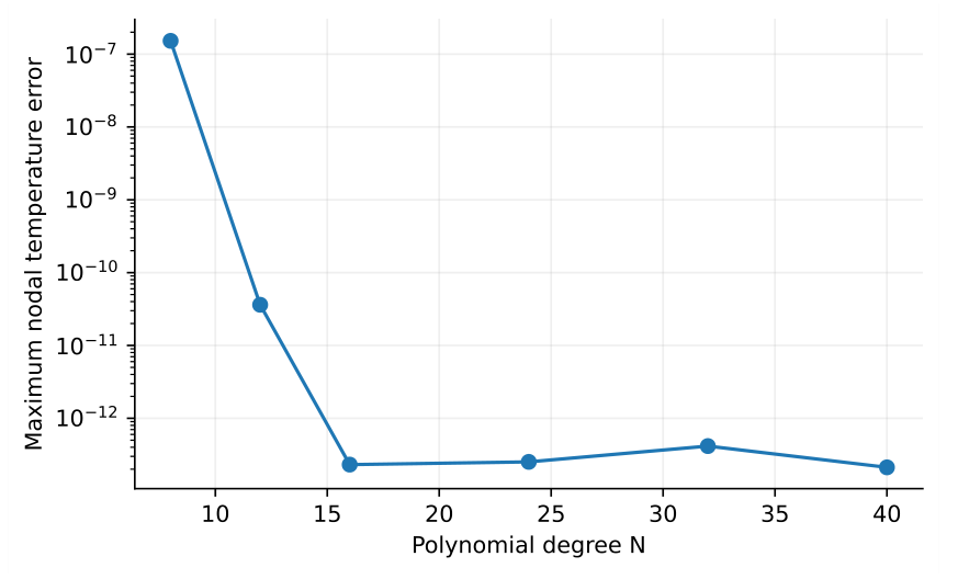
At \(N=32\), the five nonlinear Newtonian checks span \(\mathrm{Ng}=0.05\) to \(0.49\); their maximum nodal temperature error is below \(10^{-8}\). Table 2 and Figure 1 examine \(\mathrm{Ng}=0.45\). The error decreases rapidly from \(N=8\) to \(16\) and then reaches a floating-point and nonlinear-solver floor. Differentiated off-grid residuals are more sensitive to numerical cancellation and need not decrease monotonically once this floor is reached. Reporting that floor prevents roundoff-level agreement from being interpreted as unlimited accuracy.
Table 3 includes a near-turning-point Newtonian case and five sPTT cases with different sensitivities. The largest temperature difference is \(2.46\times10^{-10}\), and the largest relative Nusselt-number difference is \(3.13\times10^{-10}\). These comparisons use different meshes, residual controls, and velocity integrations. Agreement verifies the stated reduced equations, rather than validating their applicability to a specific polymer or processing experiment.
| \(N\) | \(\|\theta_N-\theta_{\rm exact}\|_\infty\) | \(\mathrm{Nu}\) | Off-grid residual |
|---|---|---|---|
| 8 | \(1.52\times10^{-7}\) | 7.815449077 | \(1.97\times10^{-5}\) |
| 12 | \(3.62\times10^{-11}\) | 7.815446748 | \(2.92\times10^{-7}\) |
| 16 | \(2.31\times10^{-13}\) | 7.815446736 | \(1.52\times10^{-10}\) |
| 24 | \(2.52\times10^{-13}\) | 7.815446736 | \(6.26\times10^{-11}\) |
| 32 | \(4.16\times10^{-13}\) | 7.815446736 | \(1.54\times10^{-9}\) |
| 40 | \(2.12\times10^{-13}\) | 7.815446736 | \(1.87\times10^{-10}\) |
| \(\mathrm{Ng}\) | \(\chi\) | \(a\) | BVP nodes | \(E_\theta\) | \(E_{\mathrm{Nu}}\) |
|---|---|---|---|---|---|
| 0.10 | 0.01 | 0.5 | 121 | \(9.13\times10^{-12}\) | \(2.85\times10^{-11}\) |
| 0.20 | 0.04 | 0.5 | 386 | \(8.51\times10^{-12}\) | \(9.66\times10^{-12}\) |
| 0.20 | 0.04 | 1.0 | 241 | \(2.95\times10^{-12}\) | \(8.83\times10^{-13}\) |
| 0.20 | 0.04 | 1.5 | 135 | \(1.06\times10^{-11}\) | \(1.66\times10^{-11}\) |
| 0.20 | 0.04 | 2.0 | 241 | \(2.46\times10^{-10}\) | \(3.13\times10^{-10}\) |
| 0.49 | 0.00 | 1.0 | 360 | \(2.93\times10^{-11}\) | \(2.57\times10^{-12}\) |
The two contributions in Eq. (8) are evaluated separately for five \(\phi\) values at \(\mathrm{Ng}=0.15\), \(\chi=0.04\), and \(a=0.5\). Each source is used in a separate solve. Table 4 reports the resulting values and their differences from \(\phi=0\). The largest temperature discrepancy is \(1.34\times10^{-14}\). This confirms the analytical invariance; it does not support a nonzero partition-induced heat-transfer correction in the present equilibrium.
| \(\phi\) | \(\theta_c\) | \(M\) | \(\mathrm{Nu}\) | \(E_\phi\) |
|---|---|---|---|---|
| 0.00 | 0.327116412 | 2.334203473 | 10.102339868 | \(0\) |
| 0.25 | 0.327116412 | 2.334203473 | 10.102339868 | \(9.83\times10^{-15}\) |
| 0.50 | 0.327116412 | 2.334203473 | 10.102339868 | \(9.94\times10^{-15}\) |
| 0.75 | 0.327116412 | 2.334203473 | 10.102339868 | \(1.34\times10^{-14}\) |
| 1.00 | 0.327116412 | 2.334203473 | 10.102339868 | \(7.72\times10^{-15}\) |
Across the 80-case production grid, the largest relative discrepancies in the integrated thermal balance and pressure-power balance are both \(2.76\times10^{-10}\). The largest normalized off-grid differential residual is \(1.20\times10^{-9}\). All validation assertions in the distributed computation script pass. The residuals, balance errors, and independent-solver differences are supplied as numerical verification measures, without a statistical or experimental uncertainty interpretation.
The production grid is the Cartesian product
All 80 combinations converge on the zero-heating-connected branch. At \(\chi=0\), changing \(a\) has no effect because the relaxation-dependent term vanishes; these repeated control cases are included in the grid count. The independent values of \(\mathrm{Ng}\) and \(\chi\) describe a model-space sensitivity study. Changing pressure in a single physical device would generally change both groups, and requires following the corresponding joint parameter path.
The source structure in Eq. (15) separates a term proportional to \(\mathrm{e}^\theta\) from the sPTT contribution proportional to \(\mathrm{e}^{(3-2a)\theta}\). At \(a=0.5\), the latter grows as \(\mathrm{e}^{2\theta}\). At \(a=1\), both terms grow as \(\mathrm{e}^\theta\). At \(a=1.5\), the sPTT contribution is independent of temperature, and at \(a=2\) it decreases as \(\mathrm{e}^{-\theta}\). This decomposition explains why the relaxation-time sensitivity can alter feedback even though viscosity always decreases with temperature.
Figure 2 shows temperature and mean-normalized velocity at \(\chi=0.04\), \(a=0.5\). Increasing \(\mathrm{Ng}\) from \(0.01\) to \(0.20\) increases the centerline temperature excess and decreases the central viscosity ratio. At \(\mathrm{Ng}=0.20\), \(\theta_c=0.547642\), \(\eta_c/\eta_w=0.578312\), and \(M=2.741610\). The larger flow rate at prescribed \(G\) also increases the pressure-work input and, by Eq. (22), the required wall cooling.
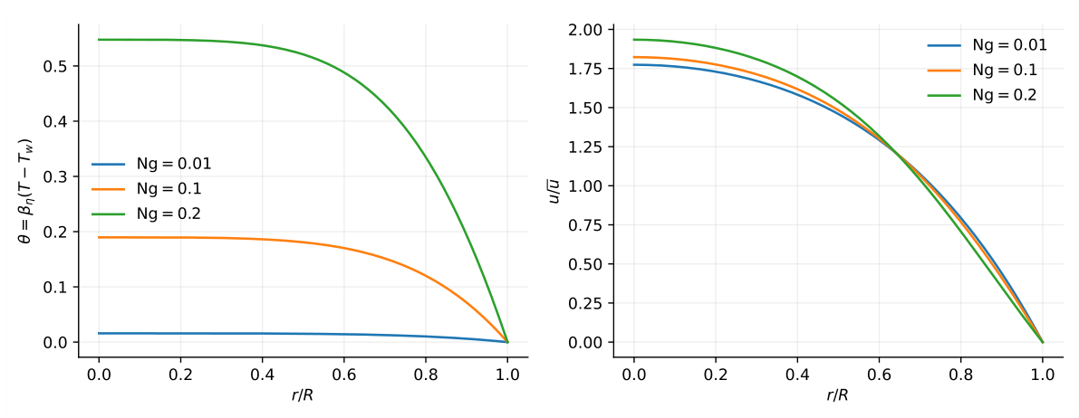
Temperature is largest at the centerline and decreases toward the wall. The zero centerline shear does not imply zero centerline temperature: heat generated at larger radii is redistributed by conduction. With \(\mathcal S\geq0\), integration of Eq. (17) establishes \(\theta_y\leq0\) for the regular solutions, consistent with the profiles.
The increase in \(M\) should be interpreted together with the normalization of the profiles. The dimensional wall shear rate remains fixed by Eq. (23), while the velocity divided by its mean changes shape. A larger temperature excess therefore need not imply a larger wall shear rate under the controls used here.
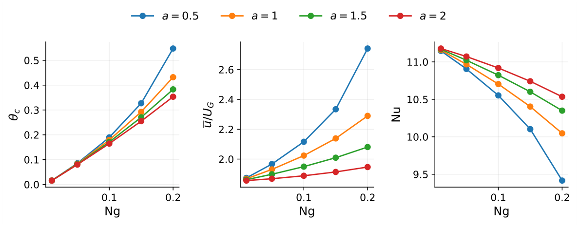
Figure 3 and Table 5 quantify the effect of \(a\) at \(\chi=0.04\). At \(\mathrm{Ng}=0.20\), increasing \(a\) from \(0.5\) to \(2\) reduces \(\theta_c\) from \(0.547642\) to \(0.353380\) and \(M\) from \(2.741610\) to \(1.946714\). The outward dimensionless flux decreases from \(2.193288\) to \(1.557371\), whereas \(\mathrm{Nu}\) increases from \(9.416165\) to \(10.534876\).
| \(\mathrm{Ng}\) | \(a\) | \(\theta_c\) | \(M\) | \(q^*\) | \(\mathrm{Nu}\) |
|---|---|---|---|---|---|
| 0.10 | 0.5 | 0.189670 | 2.116163 | 0.846465 | 10.552474 |
| 0.20 | 0.5 | 0.547642 | 2.741610 | 2.193288 | 9.416165 |
| 0.10 | 1.0 | 0.179250 | 2.023456 | 0.809382 | 10.703874 |
| 0.20 | 1.0 | 0.432096 | 2.289896 | 1.831917 | 10.046567 |
| 0.10 | 1.5 | 0.171173 | 1.949432 | 0.779773 | 10.822846 |
| 0.20 | 1.5 | 0.383071 | 2.080969 | 1.664775 | 10.349477 |
| 0.10 | 2.0 | 0.164662 | 1.888146 | 0.755258 | 10.918602 |
| 0.20 | 2.0 | 0.353380 | 1.946714 | 1.557371 | 10.534876 |
The reduction in heating reflects the faster decrease of relaxation time and the resulting attenuation of the shear-dependent contribution. The rise in \(\mathrm{Nu}\) does not mean that the absolute wall heat flux rises: \(\mathrm{Nu}\) is a ratio involving the bulk-to-wall temperature difference. Both the heat flux and its driving temperature difference must be examined before interpreting changes as an engineering improvement.
For every sampled \(a\) at \(\chi=0.04\), \(\mathrm{Nu}\) decreases with increasing \(\mathrm{Ng}\) over the tested interval. For example, at \(a=0.5\) it decreases from \(10.552474\) at \(\mathrm{Ng}=0.10\) to \(9.416165\) at \(\mathrm{Ng}=0.20\). This trend is a computed result for the present fixed-pressure, wall-cooled state. It should not be transferred unchanged to prescribed-flow-rate or wall-heating problems.
In the constant-property auxiliary limit, increasing \(\chi\) from zero to \(0.04\) raises \(\mathrm{Nu}_0\) from \(9.6\) to \(11.203150\) and increases \(M_0\) from one to \(1.853333\). Nonlinear thermal feedback modifies both quantities through Eq. (15). The relaxation and extensibility parameters enter the velocity and temperature equations through \(\chi\), so those fields alone cannot identify \(\epsilon\) and \(\mathrm{We}_G\) separately. The normal stress retains an explicit factor of \(\mathrm{We}_G\) in Eq. (13).
This distinction matters when interpreting a parameter sweep as a material characterization. The calculations determine the thermal consequences of specified model coefficients; they do not estimate those coefficients from data. Independent rheological measurements would be needed to separate the parameters and select a physically representative temperature range.
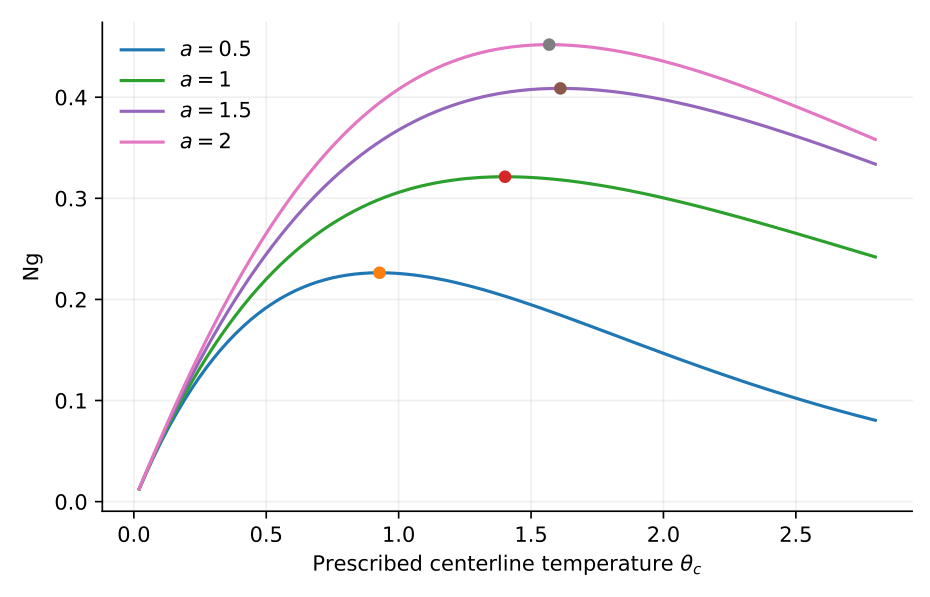
Figure 4 traces \(\mathrm{Ng}\) against prescribed centerline temperature for \(\chi=0.04\). Table 6 also includes \(\chi=0.01\) and the exact Newtonian control. The turning-point values increase with \(a\) in the tested range. At \(\chi=0.04\), they are \(0.226413\), \(0.321372\), \(0.408756\), and \(0.452037\) for \(a=0.5\), \(1\), \(1.5\), and \(2\), respectively. The Newtonian family gives \(0.5\).
| \(\chi\) | \(a\) | \(\mathrm{Ng}_{\rm turn}\) | \(\theta_{c,\rm turn}\) | \(E_{\mathrm{BVP}}\) |
|---|---|---|---|---|
| 0.00 | 1.0 | 0.500000 | 1.386294 | \(9.94\times10^{-11}\) |
| 0.01 | 0.5 | 0.379009 | 1.142132 | \(3.20\times10^{-13}\) |
| 0.01 | 1.0 | 0.439416 | 1.393050 | \(1.12\times10^{-12}\) |
| 0.01 | 1.5 | 0.471838 | 1.451003 | \(2.37\times10^{-13}\) |
| 0.01 | 2.0 | 0.485776 | 1.439813 | \(2.54\times10^{-10}\) |
| 0.04 | 0.5 | 0.226413 | 0.927550 | \(6.82\times10^{-13}\) |
| 0.04 | 1.0 | 0.321372 | 1.401592 | \(1.11\times10^{-11}\) |
| 0.04 | 1.5 | 0.408756 | 1.610713 | \(9.28\times10^{-11}\) |
| 0.04 | 2.0 | 0.452037 | 1.568357 | \(2.57\times10^{-12}\) |
For \(a=0.5\), raising \(\chi\) from \(0.01\) to \(0.04\) reduces the turning-point \(\mathrm{Ng}\) from \(0.379009\) to \(0.226413\), consistent with the stronger positive temperature dependence of the sPTT heating term. Increasing \(a\) moderates that contribution and shifts the turning point toward a larger \(\mathrm{Ng}\).
The independent adaptive turning-point calculations differ from the spectral values by less than \(2.6\times10^{-10}\) relatively. For \(\chi=0.04\), \(a=0.5\), degrees \(N=16,24,32,40\) give turning-point \(\mathrm{Ng}\) values agreeing within \(6\times10^{-13}\). The centerline location is less precisely determined by the scalar maximum because \(\mathrm{Ng}(A)\) is locally flat. Accordingly, the reported \(\theta_c\) values are rounded to six decimals, and the main conclusions rely on the better-resolved turning-point parameter.
A turning point describes the continuation geometry of steady equilibria. A statement about temporal thermal runaway, oscillations, or stability would require the time-dependent energy and constitutive equations and an eigenvalue or transient analysis. No such inference is made from failure of a fixed-parameter Newton solve or from the shape of Figure 4 alone.
The calculations constitute numerical verification of a specified continuum model. They contain no experiments, fitted polymer parameters, or measured thermal properties. The use of one mode, a linear stress function, constant conductivity, zero solvent viscosity, zero expansion, and a steady parallel velocity limits direct process prediction. A real-fluid application requires checking laminar conditions, the validity of the exponential laws, material degradation or phase changes, and the adequacy of the selected rheological model.
The source identity depends on the absence of material evolution of the stress and temperature in the adopted geometry. Developing flow, entrance regions, secondary motion, transient heating, or nonzero material-property derivatives require revisiting the full constitutive and energy transport. The present result also does not establish a global free-energy formulation for independently chosen property laws. Its thermodynamic claim is the correctly reduced energy-source equality in the stated equilibrium.
The thermal boundary condition is prescribed temperature, and the wall flux is calculated. A constant-flux formulation must include an appropriate axial thermal balance and absolute-temperature condition. The classical negligible-dissipation constant-flux value \(48/11\) consequently belongs to a different problem from the \(48/5\) benchmark used here. Distinguishing those configurations is necessary for meaningful validation.
The dataset covers a bounded parameter region and continuation interval. It does not establish a complete phase diagram, uniqueness for all coefficients, or stability of any branch. Increasing \(N\) beyond the convergence floor can amplify floating-point differentiation defects, so analytical error and off-grid residual checks should accompany any future extension to steeper profiles.
The accompanying package supplies the numerical source, exact benchmark functions, all 80 case records, independent-solver comparisons, partition checks, continued branch coordinates, turning-point convergence, and the plotted radial profiles. A single command regenerates the data and figures. Every table is generated from those CSV records. The original preliminary tables are superseded by calculations for the explicitly defined wall-cooled configuration.
The steady linear-sPTT pipe model admits an exact local equality between mechanical stress power and relaxation heating even when viscosity and relaxation time vary radially. Consequently, the reduced energy source is independent of \(\phi\) at fixed rheology. Five separately evaluated numerical partitions confirm this equality to a maximum nodal temperature difference of \(1.34\times10^{-14}\).
Prescribing the wall temperature produces a closed dissipation–conduction equilibrium. Analytical stress elimination and the squared-radius coordinate yield a compact Chebyshev formulation with an explicit centerline equation. Constant-property polynomial benchmarks, an exact nonlinear Newtonian family, independent adaptive solutions, and global heat and pressure-power balances verify the implementation. The largest conservation discrepancy over the 80-case grid is \(2.76\times10^{-10}\).
The property-sensitivity ratio controls thermal feedback through the exponent \(3-2a\) in the sPTT source contribution. At \(\chi=0.04\), \(\mathrm{Ng}=0.20\), increasing \(a\) from \(0.5\) to \(2\) lowers the centerline temperature and mean flow while raising the apparent Nusselt number. The turning-point \(\mathrm{Ng}\) on the traced steady branch increases from \(0.226413\) to \(0.452037\) over the same sensitivity range. These findings quantify steady model behaviour and identify verification targets for more general non-isothermal solvers. Their extension to transient stability and experimentally calibrated processing conditions remains a separate research task.
| Symbol | Definition |
|---|---|
| \(R,r,z\) | Pipe radius and radial and axial coordinates |
| \(u,\overline u\) | Axial and cross-sectionally averaged velocities |
| \(G=-dp/dz>0\) | Prescribed axial pressure-gradient magnitude |
| \(T,T_w,T_b\) | Local, prescribed wall, and velocity-weighted bulk temperatures |
| \(\eta_w,\lambda_w\) | Zero-shear polymer viscosity and relaxation time at \(T_w\) |
| \(\beta_\eta,\beta_\lambda\) | Temperature-sensitivity coefficients, with units \(\mathrm{K}^{-1}\) |
| \(k\) | Constant thermal conductivity |
| \(\epsilon\) | Parameter in the linear sPTT stress function |
| \(\boldsymbol\tau,\mathbf S\) | Polymeric extra-stress and rate-of-deformation tensors |
| \(\phi\) | Parameter in the reduced energy-source partition, \(0\leq\phi\leq1\) |
| \(U_G=GR^2/(8\eta_w)\) | Reference Newtonian mean velocity for the prescribed pressure gradient |
| \(x=r/R,\ y=x^2\) | Dimensionless radius and squared-radius coordinate |
| \(\theta=\beta_\eta(T-T_w)\) | Dimensionless temperature excess |
| \(v=u/U_G,\ M=\overline u/U_G\) | Dimensionless local and mean velocities |
| \(\mathrm{We}_G=\lambda_wU_G/R\) | Pressure-scaled Weissenberg number |
| \(\chi=\epsilon\mathrm{We}_G^2\) | Combined parameter governing the present flow and thermal fields |
| \(\mathrm{Ng}=\beta_\eta\eta_wU_G^2/k\) | Pressure-scaled Nahme number |
| \(a=\beta_\lambda/\beta_\eta\) | Ratio of property-sensitivity coefficients |
| \(q_w,q^*=\beta_\eta Rq_w/k\) | Outward wall heat flux and its dimensionless form |
| \(\mathrm{Nu}=2Rq_w/[k(T_b-T_w)]\) | Diameter-based apparent Nusselt number for the present equilibrium |
| \(N\) | Degree of the temperature interpolating polynomial |
Both authors contributed equally in this research.
The authors declare that there are no competing interests.
The computational source, machine-readable results, figure data, and validation summary are supplied with this manuscript. The calculations were executed with Python 3.12.14, NumPy 2.3.5, SciPy 1.17.0, and Matplotlib 3.10.8. No external experimental dataset is required.
This research received no external funding.
Generative artificial intelligence tools were used solely for language editing, grammatical correction, and improvement of readability. The author reviewed and verified the final manuscript and assumes full responsibility for its accuracy, integrity, and scholarly content.
For frozen properties, \(\mathcal S=16y+512\chi y^2\). The operator \(4(y\partial_{yy}+\partial_y)\) maps \(1-y^2\) to \(-16y\) and \(1-y^3\) to \(-36y^2\). This directly gives Eq. (32). Integrating \(v_y=-2(1+32\chi y)\) from the wall gives Eq. (31). Multiplication of these polynomials and exact integration on \([0,1]\) gives Eq. (33).
For the nonlinear Newtonian family, Eq. (34) gives
Also \(16\mathrm{Ng} y\mathrm{e}^\theta=16\mathrm{Ng} y(1+c)^2/(1+cy^2)^2\). Their cancellation requires \(\mathrm{Ng}=2c/(1+c)^2\). Define
Since \(F_c'(y)=(1+cy^2)^{-2}\), the exact velocity is
Exchanging the order of integration gives
These derivations provide direct substitution tests of the equations and independent exact values for the validation script.
From the package root, execute the following commands:
python3 code/run_study.py |
python3 code/make_tables.py |
They regenerate the CSV files, verification summary, figure PDFs and PNGs, and table fragments. Compile main.tex twice with PDFLaTeX. The Python dependency versions used for the reported run are listed in requirements.txt. The computation script stops on failed benchmark, conservation, independent-solver, or partition assertions. Automated checks are acceptance criteria for the reported model calculations and do not replace scientific assessment of the assumptions.