Oil production from a well naturally declines over time due to decreasing reservoir pressure, formation damage, and changes in reservoir–fluid properties [1, 2]. To forecast future production and estimate remaining recoverable volume, production-decline analysis—commonly referred to as Decline Curve Analysis (DCA)—has been widely applied because of its simplicity and its ability to provide rapid estimates based on historical production data [3].
The classical DCA model introduced by Arps [1] describes three types of production decline: exponential, harmonic, and hyperbolic. These models are commonly used to represent different reservoir characteristics and production behaviors, influenced by factors such as rock properties, fluid saturation, and drive mechanisms [4, 5]. However, their application may be limited under complex field conditions, particularly when production-system changes occur, such as the installation of artificial lift systems or the implementation of enhanced oil recovery methods [6].
Such modifications can violate the assumptions underlying classical decline models, leading to deviations between observed production data and DCA-based forecasts [6]. Consequently, curve-fitting techniques play an important role in adjusting decline parameters to better match actual production behavior [7]. Through statistical fitting of production data, estimated parameters can more realistically represent reservoir performance [8, 9].
In recent years, machine-learning-based approaches have also been introduced into decline curve analysis, showing improved predictive capability for both short-term and long-term production forecasting [10, 11]. Despite these developments, traditional models such as the Arps decline curves remain widely used in petroleum engineering practice, particularly for field development planning and reserve evaluation [12, 13].
Rahaman et al. [14] demonstrated that the selection of an appropriate production-decline model has a significant impact on recovery estimates and long-term production forecasts, especially in gas fields exhibiting highly variable production behavior. Similarly, Paroissin [15] proposed a stochastic formulation of Arps decline curves to explicitly account for uncertainty in production forecasting and recoverable volume estimation.
Based on this background, the present study analyzes oil-production decline in Well 15/9-F-12 of the Volve Field using a curve-fitting approach to decline curve analysis. The objective is to obtain representative decline parameters, estimate remaining recoverable volume, and provide technical support for late-life reservoir management and field-development decision-making.
The study is structured to evaluate the production performance of Well 15/9-F-12 and to forecast future production using an exponential decline model within the Decline Curve Analysis (DCA) framework. All procedures are designed to be reproducible and consistent with standard practices in decline curve analysis for technical evaluation and economic assessment.
Field production records for Well 15/9-F-12 were obtained from the Volve Field open-source dataset released by Equinor for research, study, and development purposes [16]. The dataset includes production dates, oil production rates (STB/day), periodic production volumes (bbl/month), and data-quality flags for each data point (e.g., transient, medium, and steady).
Prior to analysis, the production data were subjected to unit conversion and consistency checks, including the identification of missing values and duplicate records. Where necessary, data corrections were applied, such as calendar-day adjustments. In addition, data points affected by operational events, including shut-ins, workovers, and other production interventions, were identified and tagged. Only data representing stable natural decline behavior were selected for decline curve model fitting.
Decline segment selection aims to identify the data interval that best represents the true production-decline phase with minimal influence from operational transients. The procedure involves visual inspection of production-rate and cumulative-production curves, exclusion of periods affected by operational disturbances or anomalies, and segmentation of the dataset when shifts in production regime are identified. A decline segment is selected only if it exhibits a consistent downward trend and produces acceptable fitting residuals based on both statistical measures and visual evaluation.
Decline model selection is performed by combining physical plausibility with statistical agreement relative to the selected production data. The exponential decline model is considered when the decline rate is approximately constant, indicating stable late-time flow behavior. The hyperbolic model is evaluated as an alternative when the production data suggest a variable decline rate, which may reflect transitional flow behavior or changes in production conditions. The harmonic model is considered when the production-decline trend exhibits a very gradual late-time decline, often associated with strong boundary-dominated flow effects [17, 18].
Model verification includes a comparative assessment between the exponential model and alternative decline formulations (e.g., hyperbolic) to ensure the most appropriate representation of observed production behavior. The final model selection is based on a combination of statistical goodness-of-fit and consistency with expected reservoir performance [19].
The initial decline rate (D\({}_{i}\)) was estimated using a semi-log linear regression method under the assumption of exponential decline behavior. Historical production rate data were first screened to identify a stable declining period, excluding early-time transient effects and operational anomalies. The natural logarithm of the production rate was then plotted against time, and linear regression was applied over the selected decline window. The slope of the resulting straight line represents the negative decline rate (\(\mathrm{-}\)D\({}_{i}\)), while the intercept corresponds to the logarithm of the initial production rate. This approach provides a robust estimate of late-time decline behavior governing production forecasting and the estimation of remaining recoverable volume.
The simulation horizon extends from the final historical data point to the forecast period defined in the study, and the simulation terminates when the production rate reaches the assumed economic limit. The simulation outputs include the production-rate curve (STB/day) over time and the cumulative-production curve (MMSTB), which are used to estimate remaining recoverable volume, remaining production potential, and production life. When relevant, sensitivity analyses are performed on decline parameters and the assumed economic limit to evaluate the range of possible outcomes.
The remaining recoverable volume is calculated by cumulatively integrating the modeled production rate from the reference date to the simulation endpoint defined by the assumed economic limit. This integration represents the volume of oil expected to be produced after the reference date under the selected decline model and assumed operating conditions. The remaining recoverable volume is expressed as \(N_{rem}=\ \int\limits^{t_{end}}_{t_{ref}}{q\left(t\right)dt}\), where \(N_{rem}\ \)is the remaining recoverable oil volume at the reference date (MMSTB), q(t) is the modeled oil production rate as a function of time (STB/day), t\({}_{ref}\) denotes the reference time corresponding to the start of the forecast period, and t\({}_{end}\) represents the end of the simulation defined by the assumed economic limit.
The production lifetime is defined as the period from the final historical reference date until the production rate declines below the predetermined economic limit. It is determined directly from the simulated production-rate profile and is expressed in years and months. The analysis also considers the technical and economic implications associated with the estimated production lifetime.
Internal validation is conducted through visual and statistical comparisons between historical production data and the fitted decline curves, with residual analysis used to identify potential systematic biases. All data-selection criteria, assumptions (including the economic abandonment rate), and fitting results are clearly documented to ensure transparency and reproducibility.
To understand reservoir performance and forecast future oil flow, a detailed analysis of the production data was conducted. In this study, DCA with an exponential model was applied to production data from oil well 15/9-F-12, recorded since 1 January 2012. Petroleum Experts Integrated Production Model (IPM) software was used to process the dataset, including initial rate, decline rate, and monthly production records.
To understand reservoir performance and forecast future oil flow, a detailed analysis of the production data was conducted. In this study, DCA with an exponential model was applied to production data from oil well 15/9-F-12, recorded since 1 January 2012. Petroleum Experts Integrated Production Model (IPM) software was used to process the dataset, including initial rate, decline rate, and monthly production records. Figure 1 shows the production-rate (q\({}_{o}\)) trend over time.
As shown in Figure 1, oil production from Well 15/9-F-12 exhibits a relatively high initial rate at the beginning of 2012, followed by a short-term increase to an early peak. This behavior is characteristic of the initial production phase, during which reservoir pressure support and well conditions remain favorable. After this early peak, the production rate enters an overall declining trend.
A pronounced production drop is observed in mid-2012 in Figure 1, marked by a sharp deviation from the preceding decline pattern. Such an abrupt decrease is indicative of temporary operational effects rather than reservoir depletion, as natural decline alone would not typically produce a sudden rate reduction of this magnitude.
Subsequently, Figure 1 shows a partial recovery in production rate, suggesting that corrective operational actions or well interventions may have been implemented. Following this recovery, production continues to decline with intermittent fluctuations, ultimately stabilizing into a smoother downward trend. This late-time behavior is consistent with a mature production phase governed primarily by boundary-dominated flow conditions.
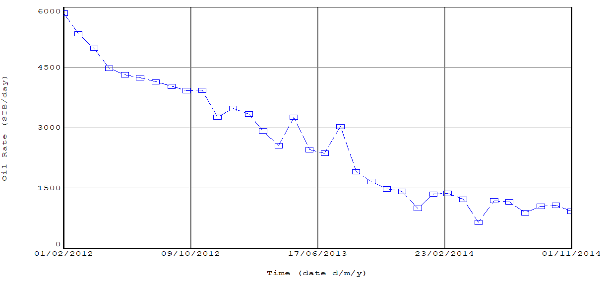
As shown in Figure 1, by 2014 the oil production rate exhibits a more pronounced decline and fluctuates within a relatively narrow range at late time. When expressed on a monthly basis, this corresponds to approximately 20,000–40,000 STB per month, indicating that the well has entered a consistent natural decline phase in accordance with DCA theory. This progressive late-time decline is characteristic of exponential or harmonic decline behavior, which are commonly applied to estimate remaining recoverable volume and well economic life.
The type of decline was determined by plotting the data on a semi-logarithmic graph, where time is displayed on a linear axis and the production rate on a logarithmic scale. When the data points form an approximately straight-line trend, the decline can be classified as exponential. Based on this semi-log analysis, the estimated exponential decline rate (Di) is 0.06. This value represents the late-time decline behavior of the reservoir and is therefore considered appropriate for production forecasting.
Long-term production forecasting was performed to characterize late-life oil-rate decline and the corresponding evolution of cumulative oil production in Well 15/9-F-12. Decline Curve Analysis (DCA) with an exponential decline model was applied to project future production behavior under mature reservoir conditions. The forecast results indicate a continuous exponential decrease in oil production rate, while cumulative oil production increases progressively and approaches an asymptotic trend, reflecting diminishing reservoir energy during the late stage of production.
As shown in Figure 2, the production forecast spans the period from 1 November 2014 to 1 June 2018. The left vertical axis represents cumulative oil production (MMSTB), whereas the right vertical axis denotes oil production rate (STB/day). Over the forecast interval, cumulative oil production increases from 0.406709 MMSTB at the reference date to 0.467232 MMSTB at the end of the simulation. During the same period, the oil production rate declines steadily from 128.896 STB/day to 9.834 STB/day, exhibiting behavior consistent with exponential decline characteristics of a late-life oil well.
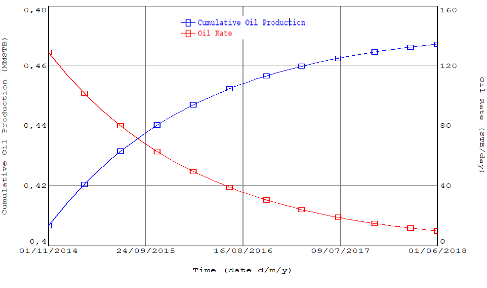
The combined trends indicate that, although the oil production rate experiences a significant and sustained decline, cumulative oil production continues to increase throughout the forecast period. The results indicate a cumulative oil production of 0.467232 MMSTB by June 2018. Starting from an initial cumulative production of 0.406709 MMSTB, an additional 0.060523 MMSTB of oil is produced during the forecast period. These findings confirm that the well is in a late-life production stage, in which the contribution of additional production progressively diminishes as the production rate approaches the economic limit. The simulated production profiles provide a quantitative basis for evaluating the remaining economic life of the well and for supporting late-life production management and abandonment planning.
Long-term production forecasting for Well 15/9-F-12 was performed using Decline Curve Analysis (DCA) with an exponential decline model to characterize oil-rate decline behavior and the corresponding evolution of cumulative oil production during the late stage of field life. The simulation results indicate that the oil production rate decreases gradually and consistently over the forecast period, while cumulative oil production continues to increase with a progressively flattening trend toward the end of the simulation, reflecting diminishing production contribution at late time.
At the beginning of the forecast period on 1 November 2014, cumulative oil production was 0.406709 MMSTB and increased steadily to 0.467232 MMSTB by 1 June 2018. This behavior is consistent with an exponential decline profile, in which cumulative oil production continues to grow over time while the contribution of additional production per unit time decreases as reservoir energy declines.
The oil-rate curve exhibits a continuous and monotonic decline from 128.896 STB/day at the start of the forecast to 9.834 STB/day at the end of the simulation period. This pronounced decline indicates that the well has entered a boundary-dominated flow regime characterized by limited reservoir support and reduced pressure energy, resulting in progressively slower production response. Concurrently, the cumulative-production curve displays a clear asymptotic tendency, indicating that the reservoir is approaching its economic production limit, where further increases in cumulative oil become marginal despite continued production time. The coupled behavior of declining oil rate and asymptotically increasing cumulative production demonstrates that the exponential DCA model provides a consistent and physically meaningful representation of late-life reservoir performance.
Based on the simulation results, cumulative oil production is projected to reach 0.467232 MMSTB by June 2018. Given a cumulative production of 0.406709 MMSTB at the start of the forecast period, the remaining recoverable volume over the forecast interval is estimated at 0.060523 MMSTB. These results indicate that, as of November 2014, the well still possessed remaining production potential; however, the magnitude of additional recovery is relatively small due to the substantial decline in oil production rate. Overall, the observed decline behavior and the limited remaining recoverable volume confirm that the well is firmly in its late-life production stage, continuing to deliver minor volumes as it approaches its economic limit.
Based on the simulation results, the economic lifetime of Well 15/9-F-12 is projected to extend until 1 June 2018, corresponding to the end of the production forecast. Referenced from the initial forecast date of 1 November 2014, this corresponds to a remaining productive period of approximately 3 years and 7 months. This duration represents the time required for the oil production rate to decline from late-life levels to values approaching the assumed economic limit, beyond which continued operation becomes marginal.
The exponential decline model applied in this study depicts a stable and continuous reduction in oil production rate, reflecting reservoir conditions that have entered a late stage of depletion. Although the production rate declines significantly over time, cumulative oil production continues to increase, as indicated by the rise in cumulative production from 0.406709 MMSTB at the start of the forecast to 0.467232 MMSTB at the end of the simulation period. This behavior confirms that cumulative production increases asymptotically while the contribution of additional production progressively diminishes, which is characteristic of exponential decline under boundary-dominated flow conditions.
The estimated economic lifetime is governed by technical parameters such as the initial forecast oil rate (128.896 STB/day), the exponential decline rate, and the assumed economic limit. The simulation results demonstrate that the well remains capable of sustained production over several years; however, the oil production rate progressively decreases and approaches 9.834 STB/day by June 2018, which is close to commonly adopted lower thresholds for economic operation. With a remaining recoverable volume of 0.060523 MMSTB over the forecast interval, the results indicate that the well still retains production potential, although the magnitude of additional recovery is relatively small compared to earlier stages of production.
The robustness of this analysis could be further enhanced by comparison with alternative estimation methods, such as analytical material balance or full-physics reservoir simulation, and by sensitivity analyses to evaluate the influence of key parameters on forecast uncertainty [22, 23]. Overall, the well-lifetime estimate derived from exponential DCA provides a sound basis for late-life technical and economic planning, including production management and abandonment considerations, and confirms that the well is in its final operational phase, delivering minor production volumes as it approaches its economic limit.
Based on the exponential Decline Curve Analysis (DCA) applied to Well 15/9-F-12, the well is confirmed to be in a late-life production stage, characterized by a pronounced decline in oil production rate from 128.896 STB/day in November 2014 to 9.834 STB/day in June 2018. Over the same period, cumulative oil production increases asymptotically from 0.406709 MMSTB to 0.467232 MMSTB, indicating that the reservoir is approaching its technical production limit under boundary-dominated flow conditions.
The analysis estimates a remaining recoverable volume of 0.060523 MMSTB at the start of the forecast period. Although additional oil production remains technically feasible, the rapidly declining production rate progressively constrains economic viability. The inferred economic limit indicates that the well remains marginally productive until approximately June 2018, implying that abandonment decisions are governed primarily by economic considerations rather than complete depletion of reservoir resources.