
Modern power electronic packages face a growing thermal problem along with device capability advancement. High-heat-flux density is becoming common due to converter size reduction, increasing switching frequency, and integration with other systems, yet volume for spreading layers, coolant pathways, and electrical isolation within packages remains limited. In the traditional thermal pathway, heat transfers from the semiconductor junction through metallized interfaces, spreader layers, lid layers, and heat exchanger into air/liquid environment. Each layer adds thermal resistance, while each interface increases complexity and thermal sensitivity to stress, interface integrity, and manufacturing process variations. This issue becomes even more challenging for SiC or GaN-based power electronics where the combination of higher switching frequency and electric field strength encourages heat generation in a small volume while junction temperature still governs reliability concerns [1– 6].
The thermal separation is mitigated in microchannel cooling systems, as the proximity of fluid flow to the heated area and greater wetted area-to-package-volume ratio enable high rates of heat transfer from a heated surface. The first silicon-based microchannel heat sink showed that the use of fine channels enables very high heat removal rates in comparison to forced convection for a liquid that flows near the heated area [7]. Subsequent work explained some of the disadvantages of this technology: small channels, which contribute to high heat transfer coefficients, may also result in higher pressure losses, increased susceptibility to inlet distribution issues, higher fouling tendency, and higher importance of manufacturing tolerances [8– 16]. Therefore, microfluidic performance cannot be determined solely on the basis of a working fluid selection. It is governed by the hydraulic diameter, wall thickness, channel pitch, manifold configuration, local Reynolds number, spreading geometry, and misalignment between the heated region and wetted region.
The designer needs to take into consideration more than just maximum power density. Any cooling system design has additional constraints related to the pressure drop, flow distribution, sealing, accessibility, mechanical integrity, electrical insulation, and economics. The examples provided by pin-fin, minichannel, and microchannel research demonstrate that higher heat transfer rate may result in increased hydraulic losses and non-uniform flows due to poorly designed inlet and outlet zones [17– 19]. Thermal interface research demonstrates that despite the effectiveness of the heat exchanger itself, poor performance can be a result of contact resistance, bond-line mismatch, pump-out effect, and/or hot spots in the thermal interface material [20, 21]. Research on multilayer spreading demonstrates that heat transfer through multiple layers depends not only on layer thickness but also on lateral heat conduction properties and the location of the heated area relative to the spreading plane [22]. There is no single figure-of-merit that captures all physical constraints of the system. Maximum power, total resistance, heat transfer coefficient, coolant volume, and marginal return all refer to different facets of the very same package level decision.
Microfluidic cooling by direct routing of the coolant to the package is a significant intermediary position between completely detached cold plates and directly machined channels within the active semiconductor material. Detached cold plates are mechanically well-known and fairly easy to maintain but leave much of the resistance from the die to the coolant in the form of package resistance. Direct-to-chip cooling reduces that distance, but may involve very delicate machining near the device. Direct routing of coolant through the package provides direct access to the coolant within the package stack yet allows more flexibility than the other approaches for assembly and material choice. This means that the routing of the coolant must be considered a thermal, mechanical, and hydraulic component of the package itself, and no longer simply an accessory [21, 23– 27].
Co-encapsulated and co-packaged cooling technologies have implications for the entire system as well. In power modules, low junction temperatures help in minimizing electrical derating and even contribute to slower fatigue of bonds, soldering layers, attachment methods, and interface materials. In data processing devices, cooling by liquids helps reduce fan energy usage while improving packaging densities, provided that the amount of energy expended in pumping the liquids, leakage prevention measures, maintenance considerations, and distribution technology stay feasible. For automotive and avionics power electronics, cooling by liquids needs to withstand vibrations, temperature changes, dielectric requirements, and long service cycles. Current research on manifolds, hybrid channels, micro-jets, and fabrication integration adds more possibilities, although each configuration comes with new distribution of thermal resistance, hydraulic pressure, and fabrication difficulties [28– 37]. The best cooling performance does not always translate into the most useful technology, which must be thermally justified.
Further examination of the literature clarifies the reason for considering the package, and not just the channel alone, as the basis for selection in this paper. Single-phase microchannels research highlights the significance of factors such as hydraulic diameter, aspect ratio, entrance development, and wall fluid interactions, whereas the two-phase microchannels’ research identifies the need to consider the trade-offs between high heat-flux capacity and pressure drop [11, 13, 38]. Demonstrations of practical silicon-based microchannels emphasize that cooler effectiveness requires the consideration of channel manufacturing, bonding, manifold connection, and pressure drop, and not just the local heat transfer coefficient [39– 41]. Solid-state thermal interfaces and materials studies lead to similar conclusions regarding the need to consider a package-level selection criteria, where even an excellent liquid flow can be limited by bond-line resistance, deterioration in the interface, and anisotropic flow through the package [21, 22, 25, 42]. This paper considers then the five tested states as a package-level flow selection problem rather than an issue of separate cooler states.
The thermal performance numbers for the states examined in this paper illustrate this trade-off very clearly. Convective air cooling delivers 6 W with a total thermal resistance of 46.42 K W−1. Liquid cooling using a heat sink with a flow rate of 30 mL/s pushes this to a maximum power delivery of 14 W while reducing the resistance to 19.30 K W−1. This comes, however, at the cost of using 3000 mL of coolant. Direct package microfluidic cooling achieves 37 W, 38 W, and 41 W for the 0.10 mL/s, 0.15 mL/s, and 0.20 mL/s flows, respectively, and uses only 2 mL to 4 mL of coolant, respectively. Corresponding values of heat flux are 578 W cm−2, 594 W cm−2, and 641 W cm−2. Those represent an important advance on air and on the separated heat sink, but also highlight a choice problem within the microfluidic system: The high-flow condition is optimal from a purely thermal standpoint; the low-flow condition is optimal in terms of heat removal per unit volume; and the middle flow condition offers modest benefit in terms of reduced resistance.
This is where thermal-resource dominance analysis can help with the decision. The method involves transforming the set of five possible conditions for the system into a unified design matrix, computing heat flux, junction-to-ambient conductance, power lift, resistance reduction, coolant economy, and resistance-normalized merit, and analyzing the microfluidic conditions by means of resistance fractioning, adjacent-flow returns, resistance leverage, preference-intervals scoring, and loading gates operation. The issue is not about liquid cooling being superior to air cooling. That much is clear from the numerical values presented earlier. The issue is narrower: What direct-to-package microfluidic flow should be maintained at each condition when the microprocessor must meet a certain heat load imposed by the maximum junction temperature with minimum use of the coolant, and why do marginal flow return and resistance partition play a key role in this respect? The outcome for each state corresponds to 0.10 mL/s as a tight, steady state, 0.20 mL/s as the peak power demand, and 0.15 mL/s as a transitional state instead of an extended stable operating condition.
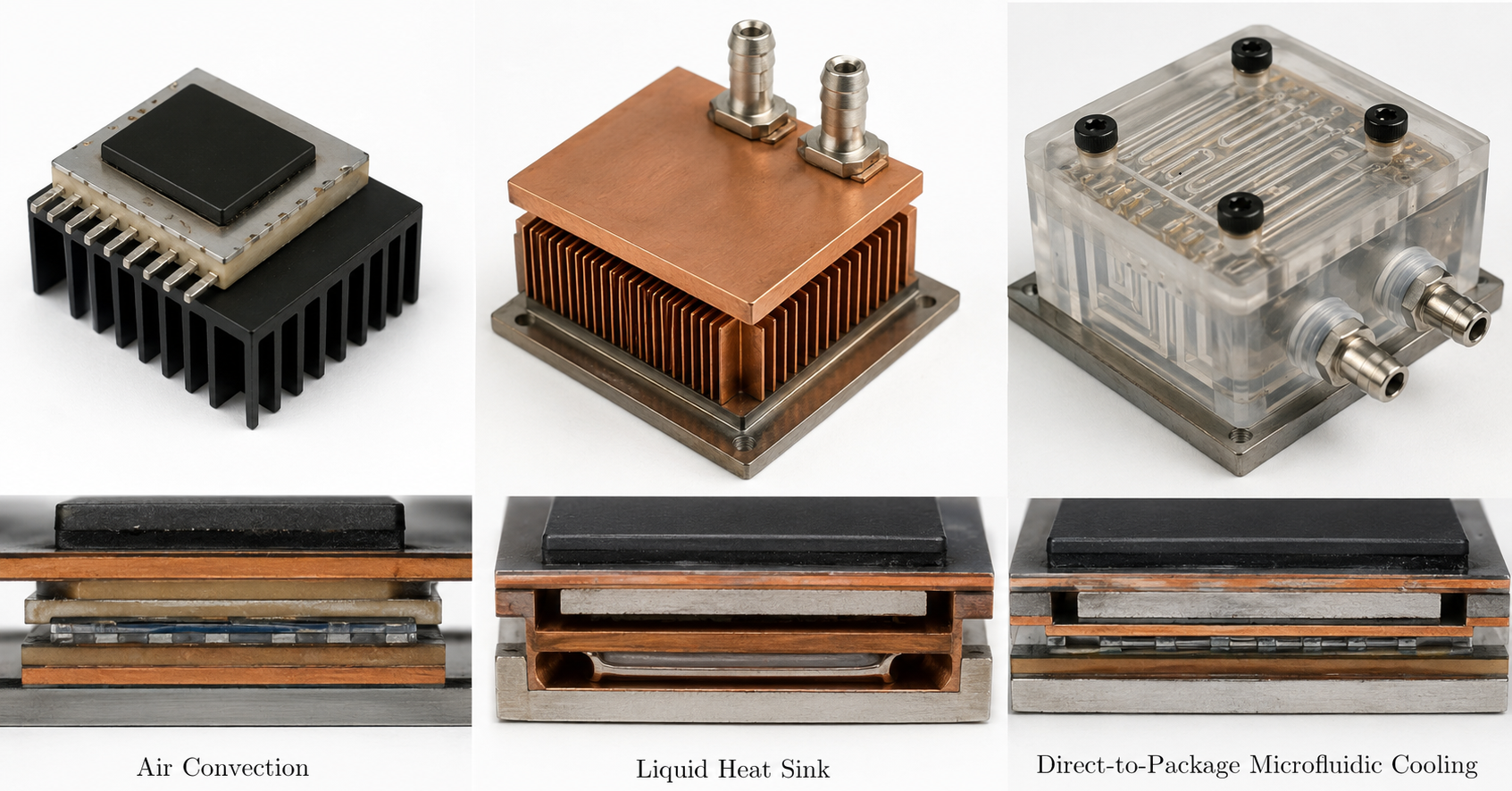
In comparison, the physical distinctions among the three types of cooling are illustrated in Figure 1, which depicts each of the three options together within a single package-level diagram.
This opening diagram provides the basis for the physical comparison. In both the air-cooling and detached heat-sink cases, a relatively large material section separates the junction from the final heat sink, while in the direct-to-package case, the liquid-cooling channel is incorporated into the package-level structure. This discussion evaluates whether the advantage still holds for the shorter path when the effects of volume and flow state are considered.
Heat sinks for a package-level system may be formulated in terms of an allocation problem, where the thermal transport path, coolant mass, and available packaging space represent competing resources. For any state \(i\), the relevant operating data may be summarized as \[\mathbf{x}_i=\left[P_{\max,i},R_{\mathrm{tot},i},V_i,f_i,h_{\mathrm{eff},i},Nu_{\mathrm{eff},i}\right]. \tag{1}\] Here, \(P_{\max}\) denotes the maximum power supported within the specified junction temperature limit, \(R_{\mathrm{tot}}\) is the overall thermal resistance from the junction to ambient, \(V\) is coolant inventory, \(f\) is volumetric flow rate, \(h_{\mathrm{eff}}\) is the overall effective heat transfer coefficient, and \(Nu_{\mathrm{eff}}\) is the overall effective Nusselt number. The vector intentionally uses a mixture of variables, including those describing absolute thermal performance, those measuring resistances, and those measuring the resource required to achieve that thermal performance state. Convection by ambient air has no liquid inventory, while the conventional heat-sink case lacks certain microfluidic resistance elements. The resulting evaluation thus separates out variables common to all three states from those relevant only to liquid-based or microfluidic states.
The maximum heat flux is obtained from the active heater area, \[q_{\max,i}=\frac{P_{\max,i}}{A_h}, \tag{2}\] and the junction-to-ambient conductance is \[G_i=\frac{1}{R_{\mathrm{tot},i}}. \tag{3}\] Considering the ambient convection regime as the benchmark, the lift in power and the reduction in resistance are written as \[L_{P,i}=\frac{P_{\max,i}}{P_{\max,\mathrm{air}}}, \qquad L_{R,i}=\frac{R_{\mathrm{tot},\mathrm{air}}}{R_{\mathrm{tot},i}}. \tag{4}\] These metrics preserve the units of the experimentally determined quantities but show the extent of improvement achieved through the switch from air cooling to either liquid cooling or microfluidic packaging. It should be noted here that these definitions have the virtue of not disguising the numbers in the list; that is, a high lift may simply be due to the high power or resistance values.
In liquid-cooled situations, the coolant economy is \[E_i=\frac{P_{\max,i}}{V_i}, \tag{5}\] which gives the allowable power per unit volume of liquid contained in the cooling solution. This value is not a substitute for pumping-power analysis, but it is an appropriate first-order indicator when the available table contains coolant volume rather than complete pressure-drop data. The resistance-corrected thermal merit is defined as \[M_i=\frac{P_{\max,i}G_i}{V_i}=\frac{P_{\max,i}}{R_{\mathrm{tot},i}V_i}. \tag{6}\] This figure favors a state only when it possesses large capacity, low overall resistance, and low coolant capacity. This is more stringent than just coolant efficiency as two states can have equal power for each milliliter but different thermal resistances resulting in different margins of temperature rise at the junction.
In microfluidic states, the overall resistance is determined by the listed terms: \[R_{\mathrm{tot},i}=R_{\mathrm{cal},i}+R_{\mathrm{conv},i}+R_{\mathrm{cond},i}. \tag{7}\] The corresponding resistance fraction is \[\psi_{\alpha,i}=\frac{R_{\alpha,i}}{R_{\mathrm{tot},i}},\qquad \alpha\in\{\mathrm{cal},\mathrm{conv},\mathrm{cond}\}. \tag{8}\] Caloric relates to the temperature increase due to the heat-carrying fluid, the convective relates to heat transfer at the wall-fluid interface and related spreading phenomena, and the conductive relates to heat transfer through the solid parts of the stack. For a dense stack, not all these terms are of equal importance. A low value for the conductive term indicates that changing the heat transfer pathway alone will have little effect, while a high convective/spreading term suggests that the location of the channels, the wetted area, and the inlet/outlet placement are important design issues.
In order to rank the three flow regimes with respect to preference continuously, we normalize the absolute values of each thermal criterion with respect to the microfluidic range. The absolute capacity index is \[A_i=0.30\widehat{P}_{\max,i}+0.25\widehat{G}_i+0.25\widehat{h}_{\mathrm{eff},i}+0.20\widehat{Nu}_{\mathrm{eff},i}. \tag{9}\] The weighting gives slightly greater weight to maximum power in consideration of typical device de-rating due to maximum heat-load allowed. However, conductance, heat transfer coefficient, and Nusselt number remain significantly weighted. Coolant economy is scaled separately as \(\widehat{E}_i\). The preference function is thus defined as \[S_i(\lambda)=(1-\lambda)A_i+\lambda\widehat{E}_i,\qquad 0\leq\lambda\leq1 . \tag{10}\] At \(\lambda=0\), the ordering is determined strictly by thermal capacity. At \(\lambda=1\), the ordering is determined strictly by coolant economy. In between, the ordering represents problems of package design where the designer places relative value on both maximum capacity and coolant economy. This structure has been deliberately chosen to accommodate other choices of weights without altering any other aspect of the analysis.
The marginal improvement in power due to an increased flow rate is measured between two successive microfluidic configurations. When the flow rate in state \(j\) exceeds that in state \(i\), the marginal improvement in power is \[\Gamma_{P,i\rightarrow j}=\frac{P_{\max,j}-P_{\max,i}}{V_j-V_i}. \tag{11}\] Analogous values are computed for heat flux, total-resistance reduction, heat-transfer-coefficient change, and Nusselt-number change: \[\Gamma_{R,i\rightarrow j}=\frac{R_{\mathrm{tot},i}-R_{\mathrm{tot},j}}{V_j-V_i}, \tag{12}\] \[\Gamma_{h,i\rightarrow j}=\frac{h_{\mathrm{eff},j}-h_{\mathrm{eff},i}}{V_j-V_i},\qquad \Gamma_{Nu,i\rightarrow j}=\frac{Nu_{\mathrm{eff},j}-Nu_{\mathrm{eff},i}}{V_j-V_i}. \tag{13}\] The positive values of \(\Gamma_P\), \(\Gamma_R\), \(\Gamma_h\), and \(\Gamma_{Nu}\) suggest that an increase in the volume of fluid leads to higher capacity, less resistance, better effective heat transfer, and increased dimensionless efficiency. The negative heat transfer value suggests that an increase in flow does not always benefit all measures of heat transfer, despite a slight increase in total power.
The Resistance Leveraging projection considers how a fractional reduction in one of the resistance components \(\eta\) will affect the measured result: \[\Pi_{\alpha,i}(\eta)=100\eta\frac{R_{\alpha,i}}{R_{\mathrm{tot},i}}=100\eta\psi_{\alpha,i}. \tag{14}\] Given a roughly constant admissible junction temperature increase, a decrease in total resistance will cause a proportional increase in allowable power with respect to the change in conductance. The estimated improvement in power due to lowering the effect of the effective convection/spreading resistance is \[\Delta P_{\max,i}^{(\mathrm{conv})}(\eta)=\Delta T_{\mathrm{allow}}\left[\frac{1}{R_{\mathrm{tot},i}-\eta R_{\mathrm{conv},i}}-\frac{1}{R_{\mathrm{tot},i}}\right]. \tag{15}\] However, the projection does not replace complete conjugate heat transfer modeling, but it provides a rigorous procedure to determine where exactly the redesign should focus within the experimentally determined resistor network.
The concept of robustness of preference refers to the dominant state for each preference level. \[i^*(\lambda)=\arg\max_i S_i(\lambda), \tag{16}\] and by computing the normalized regret of operating at state \(i\): \[\rho_i(\lambda)=\max_j S_j(\lambda)-S_i(\lambda). \tag{17}\] The mean regret over the full preference interval is \[\bar{\rho}_i=\int_0^1 \rho_i(\lambda)\,d\lambda . \tag{18}\] A low-regret state may be useful when the design preference is uncertain, even if it is not always the maximum-score state. The final selection is written in a load-gated form: \[i_{\mathrm{sel}}=\arg\min_{i\in\mathcal{F}}V_i,\qquad \mathcal{F}=\left\{i:P_{\max,i}\geq P_{\mathrm{req}},\;R_{\mathrm{tot},i}\leq R_{\lim}\right\}. \tag{19}\] The chosen strategy determines the state with the minimum coolant inventory among states satisfying the requirements on heat load and thermal resistance. This allows turning the ordinal rank ordering into a control algorithm: operate with the lowest possible coolant flow rate that satisfies the given thermal specifications, moving to higher flows only when needed by the heat load or resistance constraint.
For computations, the empirical thermal performance data reported by Martin et al. [43] are used. Numerical values presented below correspond to a heat transfer envelop for typical cooling methods, comparative performance of heat sink, direct-to-chip, and direct-to-package liquid cooling techniques, and cooling data table with maximum input power for Tj = 300 °C, total thermal resistance, effective calorimetric resistance, effective convective resistance, conductive resistance, effective global heat transfer coefficient, effective global Nusselt number, and coolant inventory. The five states considered include ambient air convection cooling and liquid cooling using heat sink, direct-to-package microfluidics with 0.10 mL/s, 0.15 mL/s, and 0.20 mL/s flow rates.
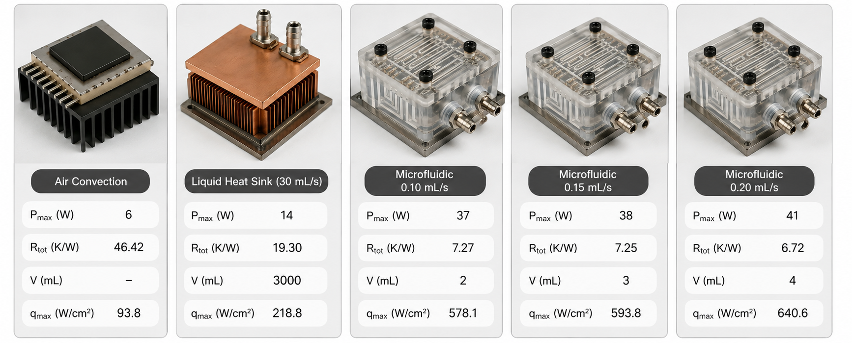
The ledger makes clear what the beginning of the analysis is. Microfluidic entries cannot be seen as just slight variations of the heat sink, but operate within a different regime that has about three times the capability in terms of heat-sink power with millilitre coolant inventory. This is the reason why the further calculations make distinction between absolute thermal capacity and relative usefulness by accounting for coolant inventory.
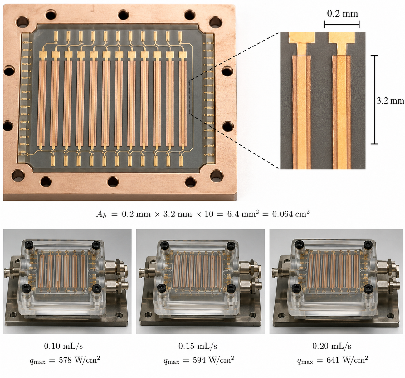
Active heat generation surface area was computed according to geometry of the heater: \[A_h=0.2~\mathrm{mm}\times3.2~\mathrm{mm}\times10=6.4~\mathrm{mm^2}=0.064~\mathrm{cm^2}. \tag{20}\] This surface was used to compute heat fluxes from maximum input power levels. Resistance and heat transfer-related quantities are already in the thermal table, which means that calculations become a straightforward interpretation at package level of all listed measures.
Geometric transformation can be seen graphically in Figure 3. There, connections between stripes on the heater and microfluidic flow states with heat-flux values were illustrated.
This is a necessary stage as the calculated maximum power values are small in watt units but are very serious when expressed per unit area of the heater. An example is 41 W which can be represented as approximately 641 W cm−2 and hence shows that the package under evaluation falls into the high heat flux category despite its overall input power level being below 50 W.
The calculations involve the following six tasks according to the thermal–resource framework. The first is the collection of the five cooling cases into a design matrix involving heat load, resistance, heat transfer, and coolant volume variables. The second task is the transformation of the design matrix to \(q_{\max}\), \(G\), \(L_P\), \(L_R\), \(E\), and \(M\). The third task entails the segregation of the three microfluidic cases into \(\psi_{\mathrm{cal}}\), \(\psi_{\mathrm{conv}}\), and \(\psi_{\mathrm{cond}}\). The fourth task consists of measuring adjacent flow transitions via \(\Gamma_P\), \(\Gamma_R\), \(\Gamma_h\), and \(\Gamma_{Nu}\). The fifth task is a resistance leverage calculation for \(\eta = 0.10\) that evaluates the influence of decreasing either the caloric, effective convective/spreading, or conductive resistance by 10%. Sixth, \(S_i(\lambda)\) is traversed for \(0\leq\lambda\leq1\), dominance intervals are established, mean regret is found, and the load-gated selection rule emerges. All these operations are based solely on the five-state matrix and the thermal properties recorded in the tables.
All computations preserve the units in the thermal table. Heat flux is in \(\mathrm{W\,cm^{-2}}\), conductance in \(\mathrm{W\,K^{-1}}\), resistance in \(\mathrm{K\,W^{-1}}\), coolant volume in mL, and heat-transfer coefficient in \(\mathrm{W\,m^{-2}\,K^{-1}}\). The water-properties and heat transfer interpretations follow the standard approach of thermal fluid analysis. Comparison of the microfluidic device with the alternative cooling modes is limited to the heat-transfer envelope defined in [44, 45]. Every numerical result reported in the results section is directly computable from the table entries and the formulas above.
The resulting design matrix is presented in Table 1. Ambient air convection can handle 6 W and has 46.42 K W−1 total resistance. Using the conventional liquid heat sink raises the maximum power to 14 W with 19.30 K W−1 total resistance, although it requires 3000 mL of coolant. The microfluidic package creates its own region on the design space graph – three different flow regimes are able to achieve 37 W, 38 W, and 41 W respectively, while total resistance is always around 7 K W−1, and the coolant volume increases from 2 mL to 4 mL. These differences explain why a liquid-cooled package cannot be considered merely a miniaturized heat sink. Both the cooling pathway and the consumption of materials change simultaneously.
Multiplying power and thermal resistances also indicates the reason why the listed states should be considered comparable despite the differences in their cooling techniques. With air convection, it results in 6 × 46.42 ≈ 278.5 K; for the heat sink it yields 14 × 19.30 ≈ 270.2 K; while microfluidic states produce 269 K, 276 K, and 276 K. As we see, they all are comparable with the thermal margin associated with Tj = 300 °C. Hence, the differences between allowable powers for these cases can be considered purely as an effect of reduction in the resistance and not as a result of increasing the temperature ceiling. It is yet another argument in favor of using resistance attenuation as a useful criterion in comparing microstates. On the other hand, it justifies why even being significantly better than air convection, the heat sink cannot outperform the direct-to-package microfluidic solution due to the long thermal path.
| Cooling state | \(f\) | \(P_\max\) | \(R_\mathrm{tot}\) | \(R_\mathrm{cal}\) | \(R_\mathrm{conv}\) | \(R_\mathrm{cond}\) | \(h_\mathrm{eff}\) | \(Nu_\mathrm{eff}\) | \(V\) |
| \((\mathrm{mL~s^{-1}})\) | (W) | \((\mathrm{K~W^{-1}})\) | \((\mathrm{K~W^{-1}})\) | \((\mathrm{K~W^{-1}})\) | \((\mathrm{K~W^{-1}})\) | \((\mathrm{W~m^{-2}~K^{-1}})\) | (– ) | (mL) | |
| Ambient air convection | – | 6 | 46.42 | – | – | – | – | – | – |
| Liquid heat sink | 30 | 14 | 19.30 | – | – | – | – | – | 3000 |
| Microfluidic package | 0.10 | 37 | 7.27 | 1.15 | 5.80 | 0.32 | 16844 | 10.41 | 2 |
| Microfluidic package | 0.15 | 38 | 7.25 | 1.09 | 5.84 | 0.32 | 16722 | 10.34 | 3 |
| Microfluidic package | 0.20 | 41 | 6.72 | 0.87 | 5.53 | 0.32 | 17672 | 10.93 | 4 |
An interesting way of looking at the design matrix is to look at the heat transfer coefficients for the microfluidic system in comparison to a general heat transfer envelope. It is seen from Table 2 that forced-liquid convection has a considerable range, and phase changes can have coefficients greater than those in the single phase, particularly in boiling and condensation where these are stable. The coefficient obtained from the microfluidic design package falls in the range of \({16722}{W\,m^{-2}\,K^{-1}}\) to \({17672}{W\,m^{-2}\,K^{-1}}\) , which is around the higher end of forced-liquid convection. The significance of this observation is that the calculated states achieve high heat transfer with no boiling involved, making resistance calculation easier and eliminating stability considerations of two phase cooling systems. The comparison also indicates that the measured performance is a consequence of proximity and wetted geometry, not merely the use of liquid water.
| Medium class | \(h\) \((\mathrm{W~m^{-2}~K^{-1}})\) | Heat-flux range at \(\Delta T={275}{K}\) \((\mathrm{W~cm^{-2}})\) |
| Free convection: gases; liquids | 2–25; 50–1000 | 0.06–0.69; 1.38–27.5 |
| Forced convection: gases; liquids | 25–250; 100–20000 | 0.69–6.88; 2.75–550.0 |
| Phase change: boiling or condensation | 2500–100000 | 68.75–2750.0 |
The heat transfer envelope table acts as a benchmark for comparison. The microfluidic data is within the upper boundary of forced liquid without phase change, so the performance advantage can be attributed to single-phase close-coupling cooling, not boiling. That is important since single-phase cooling always makes resistance partition and coolant inventory more straightforward to analyze than a two-phase mode.
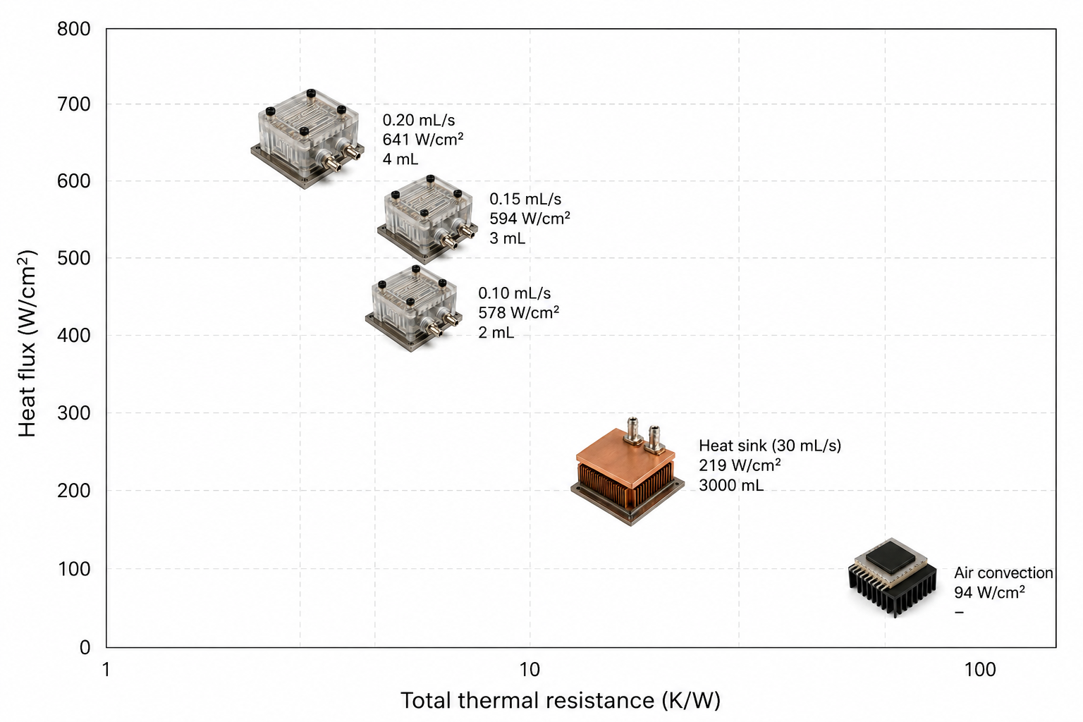
helps illustrate the distinction between the three modes of cooling using thermal dominance terrain approach. Air cooling belongs to the area of high resistance and low heat flux. The liquid heat sink is positioned at high heat flux and low resistance, but still far away from the microfluidic region. Three microfluidic points are located within a much higher conductance and heat flux zone. Besides, their closeness demonstrates another point – increment of heat flux from 0.10 mL/s to 0.15 mL/s is not observable in the resistance-capacity space, while transition from 0.15 mL/s to 0.20 mL/s results in clear improvement. Without the dominance terrain plot the relationship might have been missed out.
With regard to the terrain plot, the first major finding of the study holds true – the microfluidic cooling states are distinguished from air and detached heat sink in terms of low resistance and high heat flux values. The proximity of the three microfluidic points is another important conclusion that warns about the necessity to consider coolant inventory and marginal return when choosing flow rate within the microfluidic range.
Derived thermal and resource indicators are summarized in Table 3. With power converted to heat flux, the values are 93.8 W cm−2 for ambient convection, 218.8 W cm−2 for the heat sink, and 578.1 W cm−2, 593.8 W cm−2, and 640.6 W cm−2 for the three states of microfluidics. Thus, the heat flux for microfluidics is 2.64–2.93 times greater than that of the heat sink and 6 times greater than that of air cooling. The corresponding conductance shows similar behavior of 0.0215 W K−1 for air convection, 0.0518 W K−1 for the heat sink, and 0.1376 W K−1 to 0.1488 W K−1 for microfluidics. Power lift values of 6.17 to 6.83, along with resistance attenuation values of 6.39 to 6.91, demonstrate clearly that the introduction of a microfluidic flow at the package level influences both the permissible power dissipation as well as conductance, not at the cost of either of the indicators.
| Cooling state | \(q_\max\) | \(G\) | \(L_P\) | \(L_R\) | \(V\) | \(E\) | \(M\) |
| \((\mathrm{W~cm^{-2}})\) | \((\mathrm{W~K^{-1}})\) | (– ) | (– ) | (mL) | \((\mathrm{W~mL^{-1}})\) | \((\mathrm{W^2~K^{-1}~mL^{-1}})\) | |
| Ambient air convection | 93.8 | 0.0215 | 1.00 | 1.00 | – | – | – |
| Liquid heat sink | 218.8 | 0.0518 | 2.33 | 2.41 | 3000 | 0.0047 | 0.00024 |
| Microfluidic, 0.10 mL s\(^{-1}\) | 578.1 | 0.1376 | 6.17 | 6.39 | 2 | 18.50 | 2.5447 |
| Microfluidic, 0.15 mL s\(^{-1}\) | 593.8 | 0.1379 | 6.33 | 6.40 | 3 | 12.67 | 1.7471 |
| Microfluidic, 0.20 mL s\(^{-1}\) | 640.6 | 0.1488 | 6.83 | 6.91 | 4 | 10.25 | 1.5253 |
This yields an alternative ranking scheme. The traditional heat sink has an \({14}{W}\) cooling capability and uses \({3000}{mL^{-1}}\) of liquid, giving \({0.0047}{W\,mL^{-1}}\). The low-flow microfluidic regime cools \({37}{W}\) of power using \({2}{mL^{-1}}\) of liquid, yielding \({18.50}{W\,mL^{-1}}\). Even in the high-flow case, which has the lowest economic efficiency of the three, one achieves \({10.25}{W\,mL^{-1}}\). With correction for fluid resistance, the disparity is made even more clear: \(M = 2.5447\) in the low flow regime (\({0.10}{mL^{-1}/s}\)), \(M = 1.7471\) in the moderate-flow regime (\({0.15}{mL^{-1}/s}\)), and \(M = 1.5253\) in the high-flow regime (\({0.20}{mL^{-1}/s}\)). The high-flow regime is the most thermally efficient in an absolute sense, but the low-flow regime offers better resource efficiency.
Figure 5, displaying the inventory-normalized plot alongside its interpretation, highlights the order-of-magnitude difference between the conventional heat sink and the microfluidic package in terms of fluid inventory relative to power capacity. It should be noted that the graph does not seek to claim that all heat sinks are inherently inefficient configurations; it simply indicates that, for the present package and comparison, the volume of coolant strongly influences evaluation of thermal performance. The plot further helps to understand that the high-flow microfluidic configuration cannot be chosen only because it provides the minimum total resistance. In case where the objective for the product design is small-sized continuous operation with minimal coolant capacity, then the low-flow configuration holds more merit. However, if the heat load capacity during the shortest time period is to be maximized, then the high-flow microfluidic configuration should still be selected.
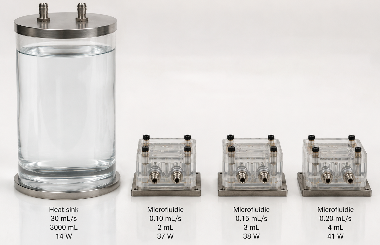
Merit ranking can also be helpful in understanding system integration. Liquid capacity may not be as critical an issue in the laboratory test environment, but it assumes more importance in a tightly integrated converter, inverter, power module, or computer data-processing node where every cubic centimeter must be distributed, contained, refilled, monitored, and serviced. The \({3000}{mL^{-1}}\) heat-sink fluid capacity thus represents a very different engineering challenge from \({2}{mL^{-1}}\) to \({4}{mL^{-1}}\) values representing fluid package integration. The latter represent relatively small capacities that can be considered within the scope of the package design, while the former represents a thermal management design outside of the package itself. This difference is also reflected by the large span of over four orders of magnitude in the resistance-corrected indicator between the conventional heat sink case and the two microfluidic cases. The indicator does not suggest that the smaller volumes are better than larger volumes. Instead, it suggests that the heat flux and compactness goals combined produce much higher thermally effective capacity in the direct-to-package states compared to conventional designs.
The second point to note about the high-flow case is the retention of absolute superiority that makes it worthwhile in spite of its extra volume in the peak load case. The coolant economy is worse than that of the low flow case but not bad in absolute terms. It is complemented by the lowest total electrical resistance, which explains the division of the design space seen in the preference analyses rather than selection of one state for all cases. The product that usually operates at around \({37}{W}\) but occasionally reaches a load of around \({41}{W}\) would be suitable for a flow controller that kept the coolant at low flow most of the time but switched to high flow just before reaching peak load. This kind of phenomenon happens quite frequently in practice when it comes to thermal management design, in which case the optimal steady-state design may differ from an optimal transient or overload design, and in which case the schedule can take advantage of both depending on controllability afforded by the package hardware.
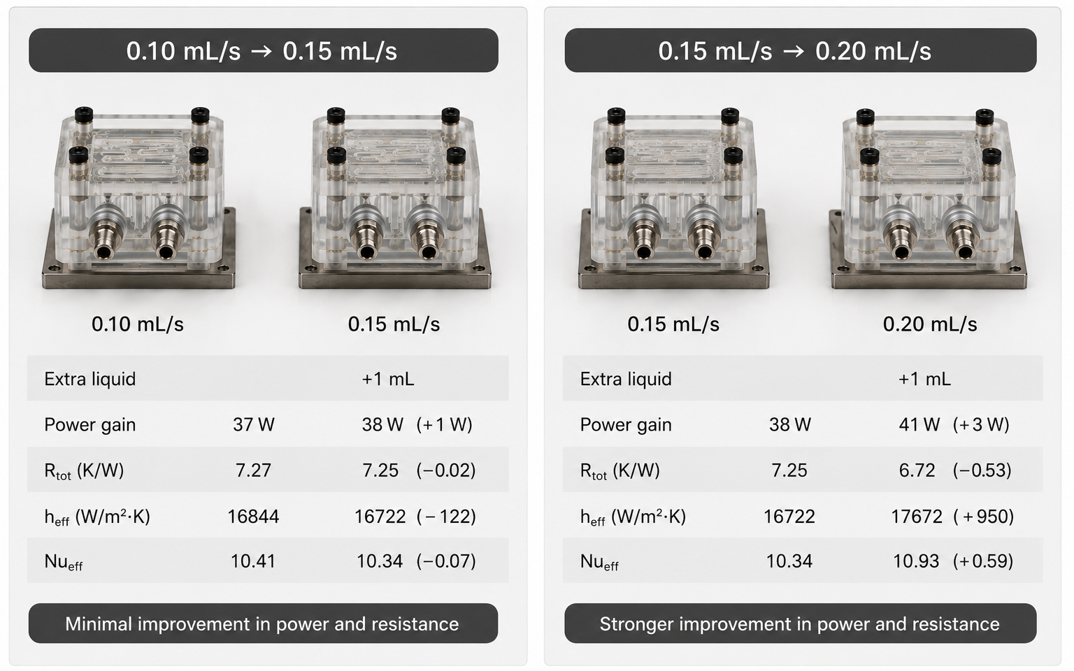
From the adjacent flow comparisons in Table 4, we note that the three operating states under consideration do not follow a strictly monotonically improved path. An increment of flow rate from \({0.10}{mL^{-1}/s}\) to \({0.15}{mL^{-1}/s}\) provides an extra \({1}{mL^{-1}}\) volume, but only a marginal increase in power capability to \({1}{W}\). The heat-flux improvement is \({15.6}{W\,cm^{-2}\,mL^{-1}}\) while the net resistance drops \({0.02}{K\,W^{-1}\,mL^{-1}}\). The more significant point to make here is that both heat transfer coefficient and Nusselt number have decreased marginally during this process. This signifies that the transitional state offers only a slight increment in power allowance without any enhancement in efficiency of the heat transfer process.
| Flow transition | Added \(V\) | \(\Gamma_P\) | \(\Delta q_\max/\Delta V\) | \(\Gamma_R\) | \(\Gamma_h\) | \(\Gamma_Nu\) |
| (mL) | \((\mathrm{W~mL^{-1}})\) | \((\mathrm{W~cm^{-2}~mL^{-1}})\) | \((\mathrm{K~W^{-1}~mL^{-1}})\) | \((\mathrm{W~m^{-2}~K^{-1}~mL^{-1}})\) | \((\mathrm{mL^{-1}})\) | |
| 0.10 \(\rightarrow\) 0.15 mL s\(^-1\) | 1 | 1.00 | 15.6 | 0.02 | -122 | -0.07 |
| 0.15 \(\rightarrow\) 0.20 mL s\(^{-1}\) | 1 | 3.00 | 46.9 | 0.53 | 950 | 0.59 |
Another scenario occurs if the flow moves from 0.15 mL s−1 to 0.20 mL s−1. In the former case, the incremental increase in liquid volume is the same 1 mL, but the gain in power return becomes 3.00 W mL−1, in heat-flux return, 46.9 W cm−2 mL−1, and in total-resistance relief, 0.53 K W−1 mL−1. In addition, the increase in effective heat transfer coefficient amounts to 950 W m−2 K−1 mL−1, while the increase in effective Nusselt number is 0.59 per mL. The greater gain in the second transition indicates that the flow distribution/thermal access reaches a more advantageous point for operation. From a product perspective, the intermediate value of flow does not qualify as an optimal steady-state position. While it could have value for smooth transitions of control or limited ranges of loads, it does not qualify to serve as an equally important reference in the design.
The picture on the adjacent-flow graph in Figure 6 presents the point more clearly. The increments in coolant volume are the same, but the increments in allowable power differ. The significance of this result is that most cooling studies present only the endpoints of the data set. This tendency can lead users to believe incorrectly that each increment in flow corresponds proportionally to an improved heat transfer capability. On the contrary, this study supports a selective approach to the flow selection. When the package dissipates less than 37 W, the low flow state is adequate for the task. For power exceeding 38 W, the high flow rate is the relevant value. Flow of 0.15 mL s−1 is only appropriate within a restricted range between the two.
The small decline in both \(h_{\mathrm{eff}}\) and \(Nu_{\mathrm{eff}}\) for the first flow level must not be viewed as a general principle of thermal conductivity law, but rather as package-level manifestation. Effective coefficients reflect the averaging impact of both local convection effect, heat diffusion influence, flow access ability and measurement reduction factor. Thus, higher nominal flow rate may fail to result in the effective increase due to extra flow bypassing active heating area, non-uniformity of temperature fields or lack of influence on critical thermal boundary layers. The powerful positive feedback in the second step implies that maximum applied flow level performs better regarding usage of added liquid. This conclusion also supports the requirement of performing flow return analysis on a package level instead of relying on channel Reynolds number only.
The presented differential analysis is important in terms of practical usage. Regular switching at unnecessarily intermediate level would result in increased activity of the pumping mechanism with no proportionate drop in junction temperature. On the other hand, making a direct step from low to high flow rate could produce significant hydraulic transients for the external loop. Intermediate flow state might still be useful as an intermediary stage of control action process, but not as preferred thermal flow state. Such differentiation is required in order not to make the design decision overly simple – one state may have important usage in control procedure without being a preferable option according to static scoring.
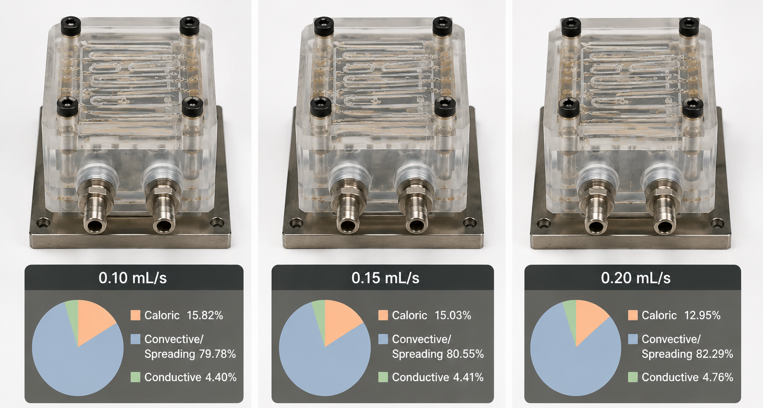
The fractions of measured resistance in Table 5 demonstrate that the convective and spreading term contributes the greatest amount of resistance in all three states of the microfluidic system. Its contribution increases from 79.78% of total resistance at \({0.10}{mL^{-1}/s}\) to 80.55% at \({0.15}{mL^{-1}/s}\) and up to 82.29% at \({0.20}{mL^{-1}/s}\). In the meantime, the fraction of resistance from caloric term gradually reduces from 15.82% to 12.95%, which correlates with the increase in liquid transport of energy at high flow. Finally, the contribution of the conductive term remains small, slightly changing from 4.40% at \({0.10}{mL^{-1}/s}\) to 4.76% at \({0.20}{mL^{-1}/s}\). Thus, the dominant role of convective/spreading term is the main advantage in the design information provided by the partition. Namely, it proves that the device is not limited by solid conduction through the stack but rather by the efficiency of liquid channel to intercept and redistribute flow around hot spots.
| Flow rate | \(R_{\mathrm{tot}}\) | \(\psi_{\mathrm{cal}}\) | \(\psi_{\mathrm{conv}}\) | \(\psi_{\mathrm{cond}}\) |
|---|---|---|---|---|
| \((\mathrm{mL~s^{-1}})\) | \((\mathrm{K~W^{-1}})\) | (%) | (%) | (%) |
| 0.10 | 7.27 | 15.82 | 79.78 | 4.40 |
| 0.15 | 7.25 | 15.03 | 80.55 | 4.41 |
| 0.20 | 6.72 | 12.95 | 82.29 | 4.76 |
The resistance-fraction table changes the design emphasis. Conductive resistance remains nearly fixed at \({0.32}{K\,W^{-1}}\), while the effective convective/spreading term stays above \({5.5}{K\,W^{-1}}\) in every microfluidic case. A package redesign that ignores this dominant term would therefore leave most of the measured resistance untouched.
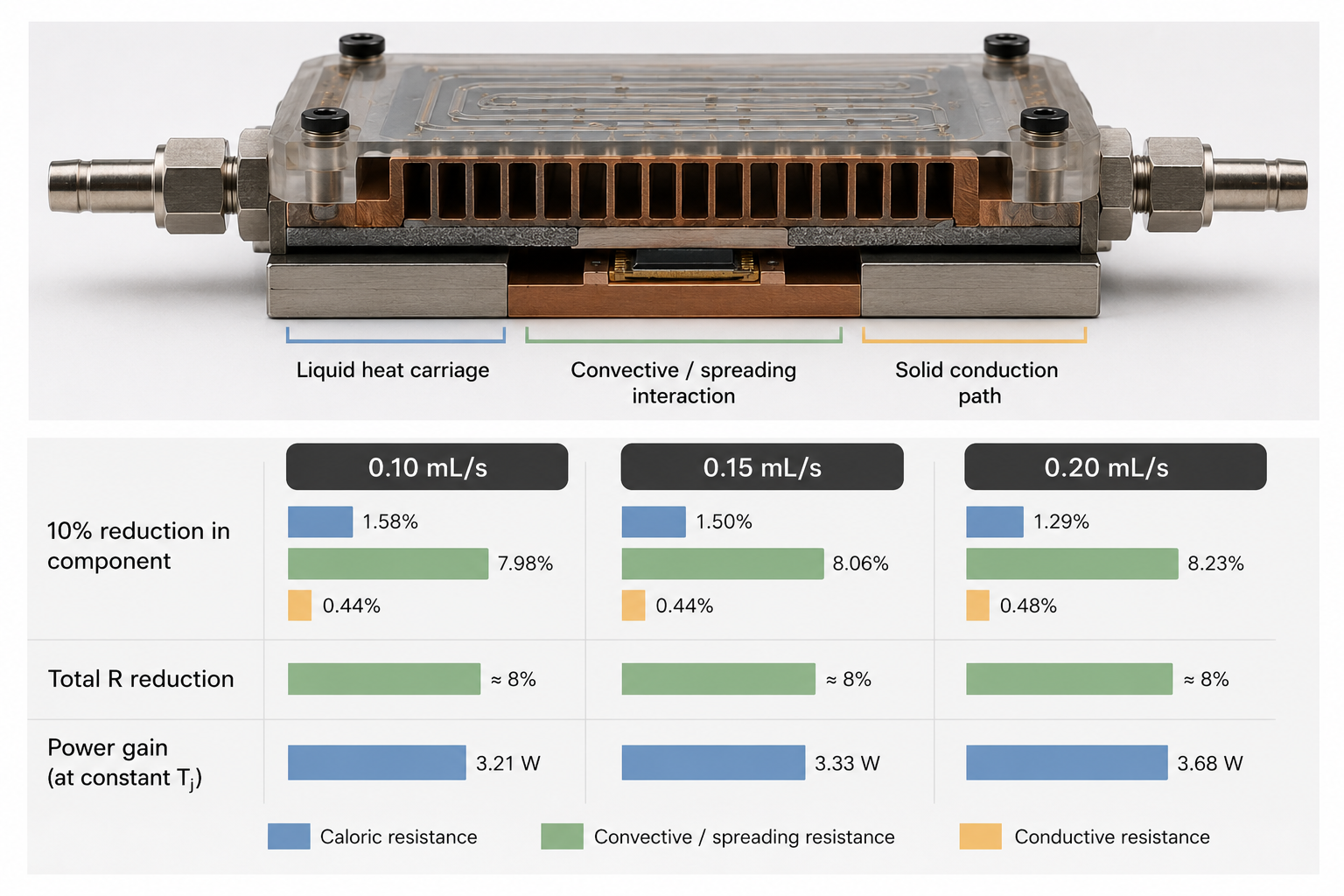
The resistance anatomy in Figure 7 presents the same resistance partition as a physical device-level anatomy, making clear that the effective convective/spreading term is the dominant resistance reservoir in all three flow states.
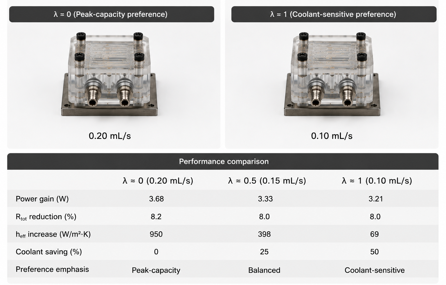
The resistance-leverage projection results are presented in Table 6 at \(\eta=0.10\). The 10% decrease of the convective/spreading effect decreases the total resistance around 8% for all examined microfluidic flow rates. If the proportionally reduced caloric contribution is assumed, then the total resistance drops by 1.29%-1.58%. The decrease of total resistance due to a 10% decrease in the conduction contribution is below 0.5%. The power savings of the constant-temperature regime from a 10% decrease of the dominating convective/spreading contribution are 3.21 W, 3.33 W, and 3.68 W at flow rates equal to 0.10 mL s\(^{-1}\), 0.15 mL s\(^{-1}\), and 0.20 mL s\(^{-1}\), respectively. The obtained savings are similar or exceed the observed power increment between neighboring flow rates. Thus, improving the wetted geometry can be as beneficial as an increment of the operation flow rate.
| Flow rate | \(\Pi_{\mathrm{cal}}(0.10)\) | \(\Pi_{\mathrm{conv}}(0.10)\) | \(\Pi_{\mathrm{cond}}(0.10)\) | \(\Delta P_{\max}^{(\mathrm{conv})}(0.10)\) |
|---|---|---|---|---|
| \((\mathrm{mL~s^{-1}})\) | (%) | (%) | (%) | (W) |
| 0.10 | 1.58 | 7.98 | 0.44 | 3.21 |
| 0.15 | 1.50 | 8.06 | 0.44 | 3.33 |
| 0.20 | 1.29 | 8.23 | 0.48 | 3.68 |
The leverage plate in Figure 8 connects the resistance fractions to practical intervention zones and projected power gains, translating the partitioned resistance table into a package-level redesign priority.
While the leverage calculation implies some modifications in terms of the package itself, such as increasing the wetted area under the heater stripes, decreasing the non-wetted area, increasing symmetry of the inlet-outlet geometry, optimizing the channel pitch, and eliminating stagnation regions, these will likely lead to a reduction in total resistance rather than the thickening of an already thin resistance layer. Such considerations follow naturally from the literature dealing with microchannel and embedded cooling, in which local flow pattern optimization and alignment between the heater and manifolds play important roles despite the good thermophysical properties of the liquid [26, 27, 31, 36, 40, 41]. It means that future designs with direct-to-package cooling would benefit from having both the thermal measurement along with some form of flow visualization, or validated conjugate simulation, which would allow the effective convective/spreading term to be broken down into wall-to-liquid heat transfer, lateral conductive, and flow non-uniformity contributions.
In addition, the relative contributions of each resistive component explain why simply boosting flow rate will at some point become less effective. Flow enhancement implies reducing the caloric term’s fractional contribution, meaning the coolant temperature effect is being mitigated. The convective/spreading term dominates, and its fractional contribution is increased. In other words, once this becomes the dominating factor, further flow will have decreasing efficiency without improving the geometry’s capability to facilitate the thermal interaction between the walls and coolant. This is what the leverage prediction represents in terms of practical consequences. Instead of working the package harder, it makes sense to modify the package design to ensure better thermal accessibility of the heated zone by the fluid.
When it comes to manufacturing, the implication is that channel topology should always be evaluated considering assembly tolerance. While tighter channel spacing could increase surface area, it could simultaneously lead to higher pressure drop, greater susceptibility to contamination issues, and difficulty in filling. A larger manifold could improve the uniform distribution, but the extra space would be used for electrical or mechanical insulation. An increase in the thickness of the conductive spreading plane is likely to mitigate hot spots, but the conductive fraction from measurements indicates it is not a limiting factor currently. The most promising next step would involve comparing alternative channel geometries that change coverage and distribution while maintaining the heater size and maximum temperature constant.
The preference horizon shown in Figure 9 is an overlay of absolute-capacity index on normalized coolant economy, forming a preference-switch horizon. In the region where \(0\leq\lambda<0.486\), the high-flow configuration is dominant because peak thermal capacity takes the heavier design weight. In the other part where \(0.486<\lambda\leq1\), the low-flow configuration is dominant because coolant economy is weighted enough to counterbalance the smaller heat-transfer index. The intermediate state will never become the dominant state because it falls between the two anchor states in terms of flow rate and coolant volume. Such absence of dominance interval agrees well with the conclusion drawn from differential analysis: \({0.15}{mL^{-1}/s}\) is a transition state, not a preferred optimum.
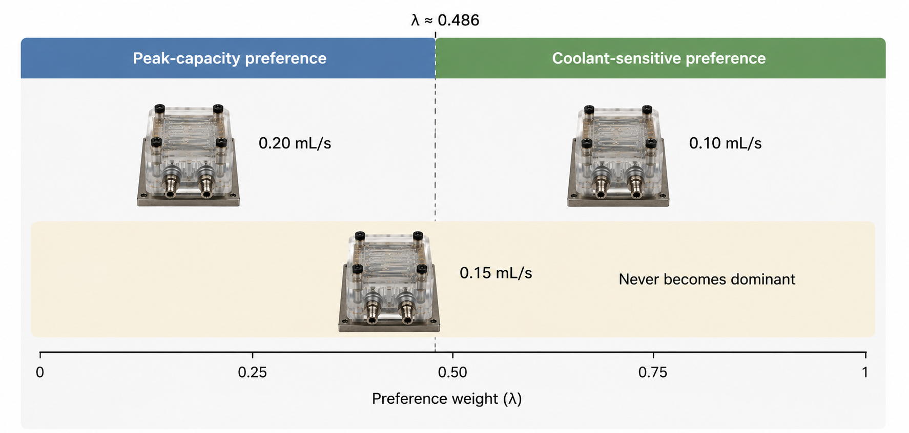
The domination intervals and regret values of each state are presented in Table 7. In particular, the low-flow state dominates 51.4% of the interval of preferences and has the minimum value of mean regret, \(\bar{\rho}=0.229\). The high-flow state dominates 48.6% of the interval of preferences and has a marginally higher value of mean regret, \(\bar{\rho}=0.257\). The intermediate flow state does not dominate any interval and has a relatively large value of mean regret, \(\bar{\rho}=0.569\). This information can be used in the practical sense because usually, preference functions in product design problems are not known precisely and rigorously. If the design team does not know for certain what to expect from the coolant economy, it is safer to start with the low-flow state since it works well enough in the most coolant-sensitive part of the preference domain and remains feasible for the range of heat loads up to \({37}{W}\). On the other hand, the high-flow state should be chosen consciously when there is a need to increase the power load or decrease the thermal resistance.
| Flow rate | \(A_i\) | \(\widehat{E}_i\) | Dominant \(\lambda\) interval | Dominance span | Mean regret \(\bar{\rho}_i\) |
| \((\mathrm{mL~s^{-1}})\) | (– ) | (– ) | (– ) | (– ) | (– ) |
| 0.10 | 0.056 | 1.000 | \(0.486<\lambda\leq1\) | 0.514 | 0.229 |
| 0.15 | 0.083 | 0.293 | none | 0.000 | 0.569 |
| 0.20 | 1.000 | 0.000 | \(0\leq\lambda<0.486\) | 0.486 | 0.257 |
The score boundary can also be read as a design-negotiation tool. When \(\lambda\) is below the boundary, the designer is effectively saying that the package should prioritize peak heat-load tolerance, even if more coolant inventory is required. When \(\lambda\) is above the boundary, the designer is saying that compactness and liquid minimization are sufficiently important to accept a lower maximum power. Because the boundary lies close to the middle of the interval, neither criterion is negligible. The package has two credible anchors rather than one overwhelming winner. This is a useful outcome for engineering decision making because it makes the trade-off explicit. A thermal engineer can recommend the high-flow state for worst-case operation, while a packaging engineer can defend low-flow operation during ordinary service without contradicting the measured data.
The mean-regret values add another practical layer. Regret is small when a state remains close to the best score across many preference values and large when a state performs poorly outside a narrow philosophy. The low-flow state has the lowest mean regret because it is extremely strong when coolant economy matters and not catastrophically weak when absolute capacity matters. The high-flow state has slightly higher regret because its score declines as the design becomes more coolant-sensitive, yet it remains essential in the peak-capacity region. The intermediate state performs poorly because it is neither the strongest thermal state nor the most economical state. This quantitative result supports the qualitative engineering intuition that middle settings are not automatically balanced settings; they can also be compromised settings.
The load-gated rule in Table 8 converts the ranking into an operating recommendation. For \(P_{\mathrm{req}}\leq{37}{W}\) and \(R_{\lim}\geq{7.27}{K\,W^{-1}}\), \({0.10}{mL^{-1}/s}\) is selected because it satisfies the thermal requirement with the smallest coolant volume. The \({0.15}{mL^{-1}/s}\) state is selected only for \({37}{W}<P_{\mathrm{req}}\leq{38}{W}\) with \(R_{\lim}\geq{7.25}{K\,W^{-1}}\). For loads above \({38}{W}\) and up to \({41}{W}\), or for a resistance requirement as low as \({6.72}{K\,W^{-1}}\), \({0.20}{mL^{-1}/s}\) is selected. If the required power exceeds \({41}{W}\), or if the allowable resistance is below \({6.72}{K\,W^{-1}}\), none of the tested states satisfies both constraints. The operating set then reaches its limit, and the channel geometry, wetted area, package stack, or coolant path must be changed. The score boundary is also a design negotiation method. For \(\lambda < \Lambda^*\), the designer is saying that peak capacity must be maximized, even at the expense of increased coolant inventory. For \(\lambda > \Lambda^*\), the designer is saying that compactness and reduced liquid volume are priorities that are worth accepting a decrease in peak power. As the boundary is close to the midpoint of the interval, neither is trivially ignored. The package has two reasonable criteria instead of one dominant design principle. This can be useful information for the engineer because it highlights the clear trade-offs involved. One engineer can advocate high flow rates in extreme cases where high heat load is expected while another engineer can support low flow rates under normal conditions without conflicting with the actual measurements.
The mean regret values provide additional insights on practical grounds. There is less regret when the state score stays near its optimal value regardless of the preferences while there is greater regret when the state’s score is poor despite being far from its optimal preferences. The low-flow state has the least mean regret because it is an excellent state for coolants sensitive designs and is not particularly bad for peak capacity. The high flow rate design is slightly better in regret because its score decreases with coolant sensitivity while still remaining necessary for peak capacity. However, the intermediate state is poor because it is not good in terms of peak capacity and coolant saving. This quantitative result supports the qualitative engineering intuition that middle settings are not automatically balanced settings; they can also be compromised settings.
The load-gated rule in Table 8 converts the ranking into an operating recommendation. For \(P_{\mathrm{req}}\leq{37}{W}\) and \(R_{\lim}\geq{7.27}{K\,W^{-1}}\), \({0.10}{mL^{-1}/s}\) is selected because it satisfies the thermal requirement with the smallest coolant volume. The \({0.15}{mL^{-1}/s}\) state is selected only for \({37}{W}<P_{\mathrm{req}}\leq{38}{W}\) with \(R_{\lim}\geq{7.25}{K\,W^{-1}}\). For loads above \({38}{W}\) and up to \({41}{W}\), or for a resistance requirement as low as \({6.72}{K\,W^{-1}}\), \({0.20}{mL^{-1}/s}\) is selected. If the required power exceeds \({41}{W}\), or if the allowable resistance is below \({6.72}{K\,W^{-1}}\), none of the tested states satisfies both constraints. The operating set then reaches its limit, and the channel geometry, wetted area, package stack, or coolant path must be changed.
| Thermal request and resistance allowance | Selected state | Design interpretation |
| \(P_\mathrm{req}\leq{37}{W}\), \(R_\lim\geq{7.27}{K\,W^{-1}}\) | \({0.10}{mL^{-1}/s}\) | Minimum coolant inventory with high inventory-normalized merit. |
| \({37}{W}<P_\mathrm{req}\leq{38}{W}\), \(R_\lim\geq{7.25}{K\,W^{-1}}\) | \({0.15}mL^{-1}/s\) | Feasibility bridge for a narrow load band; not a broad optimum. |
| \({38}{W}<P_\mathrm{req}\leq{41}{W}\), \(R_\lim\geq{6.72}{K\,W^{-1}}\) | \({0.20}mL^{-1}/s\) | Peak-capacity state with highest heat flux and lowest total resistance. |
| \(P_\mathrm{req}>{41}{W}\) or \(R_\lim<{6.72}{K\,W^{-1}}\) | No tested state satisfies both constraints | Channel topology, wetted coverage, or package-stack design must be changed. |
The solution presented by the load-gated table provides a straightforward engineering solution to the selection problem. The table does not rate the states according to some numerical criterion; rather, the load-gated solution selects the lowest flow state capable of satisfying the given load and resistance criteria. In this manner, unnecessary cooling water is not consumed under moderate loads, and the high-flow state is retained exclusively in the one area where increased inventory makes sense.
As shown in Figure 10, an equivalent solution appears on the operating map in the form of the rule “select the minimum coolant inventory to meet the necessary load and resistance criteria.”
The last note to make, with respect to comparing the standard heat sink against the microfluidic states based on heat flux rather than maximum power alone, is the following. The standard heat sink gets up to \({218.8}{W\,cm^{-2}}\) of heat flux, which is no mean feat compared with the maximum for air, but the lowest of all microfluidic states reaches a heat flux of \({578.1}{W\,cm^{-2}}\) while utilizing a coolant volume three orders of magnitude lower. The high-flow state achieves \({640.6}{W\,cm^{-2}}\), nearly the limit of the forced-liquid regime. Therefore, in addition to being compact, the benefit of a microfluidic path at the package level is that it alters the class of heat flux possible for the package. Packages that would otherwise have to use an external cold plate can operate under substantially higher heat flux conditions due to placing the liquid closer to the source of heating.
This does not detract from the need for caution, even with respect to what has been shown thus far. There is a difference between coolant volume and total cost for a system that includes a pump, potential leakage rates, pressure drops, acoustic noise, ease of filling, field-serviceability, and materials compatibility over time. The former do not impact the conclusions here because they define the range of applicability. The choice of microfluidic states is based solely on the information in the thermal table. A complete product qualification would involve adding criteria based on hydraulics, mechanics, electrical isolation, and reliability. The dominance map can accommodate such criteria in the future.
This comparative exercise serves an instructional role in terms of the design of packages. Even though the heat sink uses a greater coolant inventory, it does not come close to the microfluidic package in terms of heat flux and resistance. This does not necessarily imply that liquid cooling is irrelevant in packaging; it implies that the thermal pathway and package design for liquid cooling are different from that of the microfluidic approach. The former will be preferred when serviceability and low manufacturing risks are critical considerations. However, the latter approach can be preferable if heat flux, volume restrictions, and limited coolant availability prevail. Thus, this comparison suggests the necessity for conditional design recommendations in contrast to rankings of various cooling techniques.
As seen from the above, a heat transfer coefficient is far from being a sufficient parameter in selecting between the two states. As already mentioned above, the high-flow state possesses maximum values of both effective heat transfer coefficients and Nusselt numbers. At the same time, the low-flow state provides higher efficiency in terms of coolant consumption and the performance factor corrected by resistance. If designers focused solely on maximum heat transfer coefficient, they would inevitably opt for the high-flow state. On the contrary, if they were interested in maximum coolant efficiency, they could easily neglect the superiority of high flow rates in terms of resistance and heat flux.In other words, this is the trade-off between efficiency and effectiveness that is clearly quantified by the preference boundary near \(\lambda\approx0.486\).
Here are a few recommendations for future design efforts based on the analysis results. Further work should be done to optimize the current design to improve liquid penetration of the heating area, redesign channels under heater stripes, remove dead zones, and engineer better manifolds to deliver a uniform flow without creating a large pressure drop. If future testing campaigns will involve parameters like pressure drop, pump energy consumption, liquid leakage detection, temperature cycling and dynamic behavior, the existing dominance map can be easily extended to take these additional factors into account. It is worth noting that such an extension would also be aligned with the general direction of current electronics cooling studies [1, 23, 27, 31, 34, 35, 36].
The example with the five-state decision demonstrates how to interpret the results of a comparative evaluation when multiple states exist. Based on the peak power output, we have found that \({0.20}{mL^{-1}/s}\) is the best thermal performance. However, taking into account the coolant economy and resistance-adjusted merit, we can conclude that \({0.10}{mL^{-1}/s}\) would be the most efficient steady-state value. Meanwhile, the middle value still cannot be recommended as a design solution since it requires consuming \({3}{mL^{-1}}\) per second and delivering just \({1}{W}\) more compared to \({0.10}{mL^{-1}/s}\). In this case, any increase in thermal performance is reasonable if it contributes to increased cooling capacity, reduction of resistance, or an increase in the heat transfer coefficient.
Furthermore, the analysis defines the limits of the envelope under test. No states should be applied beyond \({41}{W}\), since no further testing or validation of the thermal model has been performed at higher power levels. While the high-flow state is the most optimal of the tested states, it is far from sufficient to imply that additional heat will be absorbed simply through the addition of flow. The dominant convective/spreading resistance represents a geometry-driven limitation and, in general, geometry-driven limitations require a change in design rather than merely a change in operational point. This is relevant to power electronics due to the typical behavior of loads to increase after the packaging of the cooling device. The load-gated rule provides clarity on this matter by defining a precise limit of load where a new design becomes necessary.
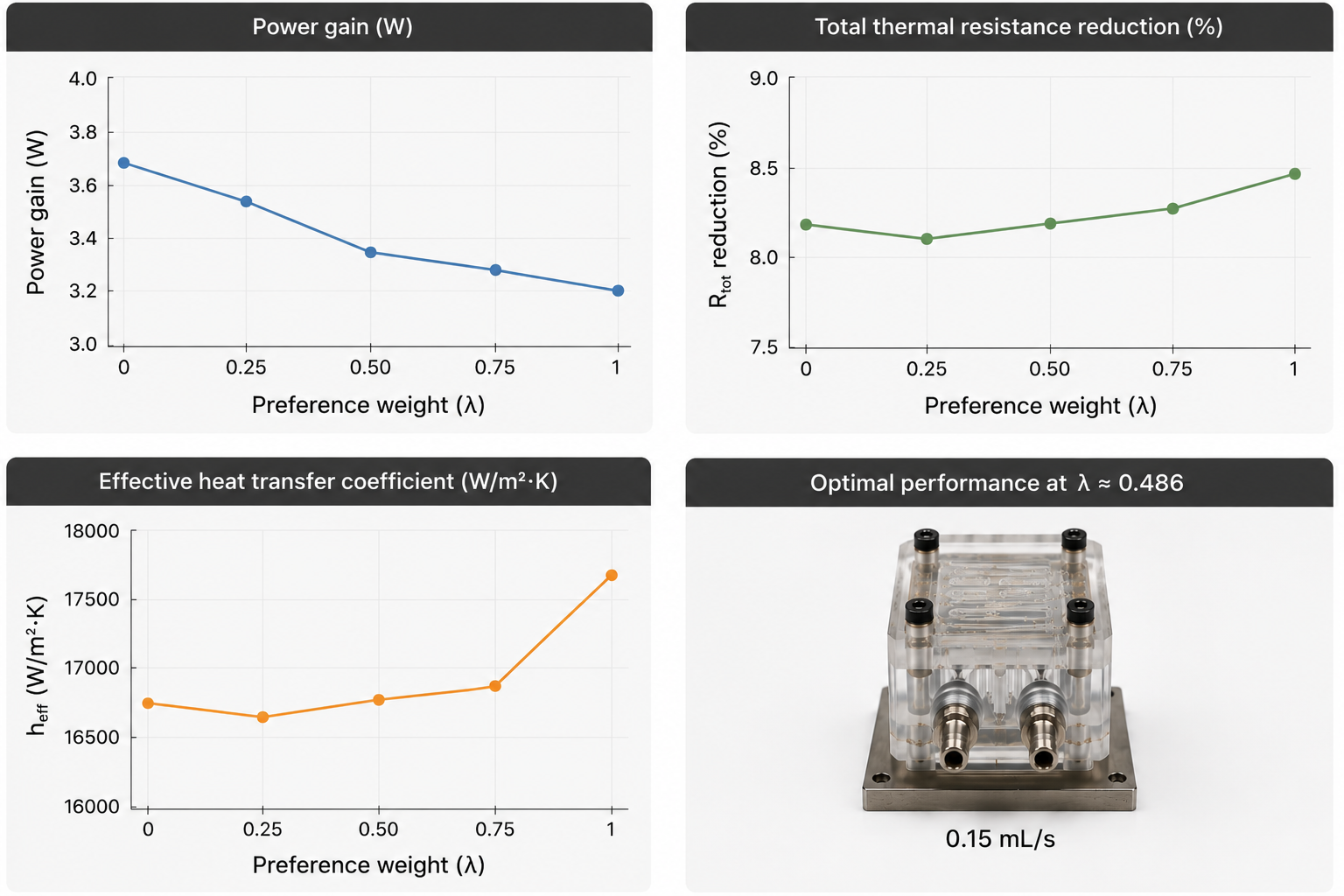
Figure 11 shows the microfluidic selection verdict plate, which provides insight into the flow states’ performance prior to applying the final rule to determine the need for design change.
This visual conclusion summarizes the findings of the paper without presenting an additional step of analysis. It is clear that the low-flow state remains a compact steady choice; the high-flow state is kept for peak performance, while the intermediate state is downgraded to the transition one since its larger coolant inventory cannot compensate for any extra thermal benefit.
This study answered the question about which of three possible direct-to-package microfluidic flow states would be appropriate when maximum heat-load capacity, total resistance, coolant inventory, marginal flow return, and resistance composition were all analyzed under the same junction-temperature constraint. The optimal answer is not a universal flow rate. Two feasible operating anchors of the tested package are 0.10 mL s−1 (compact steady state) and 0.20 mL s−1 (peak state). The third one (0.15 mL s−1) fails to become an optimum due to its higher coolant inventory producing only extra 1 W of heat capacity and minor total-resistance reduction relative to 0.10 mL s−1.
The numerical solution is exact and traceable. Air convection is capable of removing 6 W at 46.42 K W−1, while the detached heat sink removes 14 W at 19.30 K W−1 with 3000 mL of coolant. The direct-to-package microfluidic states provide 37 W, 38 W, and 41 W, respectively, but use just 2 mL, 3 mL, and 4 mL. Based on the pure thermal capability, the 0.20 mL s−1 state is most powerful: it achieves approximately 641 W cm−2, exhibits minimal total resistance of 6.72 K W−1, and shows maximal heat-transfer coefficient and Nusselt number. In terms of the coolant economy, the 0.10 mL s−1 state prevails: it achieves approximately 578 W cm−2 with only 2 mL coolant and gives maximal coolant economy and merit.
From the resistance perspective, the reason why simply boosting the flow rate is not enough becomes clear. The effective convective/spreading term represents around 80-82% of total resistance, while the conductive term remains below 5%. The key issue here is the implementation of the wetted surface beneath the heated area in terms of location and utilization: the channel pitch, inlet/outlet ratio, flow distribution, and lateral heat-spreading through the liquid-contact area. Thus, the preference boundary for \(\lambda \approx 0.486\) means that peak capacity selects 0.20 mL s−1 below it, while coolant-sensitive package design prefers 0.10 mL s−1 above it. Practically, this leads to load-gating: running the package with 0.10 mL s−1 when the load is less than 37 W and the resistance limit is greater than 7.27 K W−1, using 0.20 mL s−1 for 38 W–41 W loads or tight resistance requirements, and redesigning the package in case of a larger load than 41 W or lower resistance limit than 6.72 K W−1.