As environmental awareness and energy conservation consciousness continue to grow, many large and medium-sized enterprises, such as steel and metallurgy, petrochemical, and thermal power plants, have increasingly prioritized improving furnace thermal efficiency, reducing energy consumption, lowering pollutant emissions, and protecting the environment as key strategies for sustainable corporate development [1– 4]. Combustion devices and thermal engineering equipment such as rolling mill heating furnaces in the steel industry and boilers in the power industry are major energy consumers across various industries [5, 6]. Therefore, measuring and improving the combustion efficiency of combustion devices and determining the optimal combustion point are of great importance.
For fuel-fired industrial furnaces, fuel combustion efficiency and fuel utilization efficiency are two critical technical and economic indicators [7]. Fuel combustion efficiency reflects the degree of fuel combustion, which can be evaluated by analyzing the composition of combustion products to calculate parameters such as combustion completeness, residual oxygen content, and excess air coefficient, thereby determining whether the furnace is operating at optimal combustion conditions [8– 10]. Fuel utilization efficiency reflects the extent to which the heat released by fuel combustion is effectively utilized. The higher the fuel utilization efficiency, the lower the fuel consumption or thermal consumption of the furnace or kiln [11– 13]. High utilization efficiency first requires high combustion efficiency as a prerequisite [14]. Monitoring these two indicators enables furnaces and kilns to operate in optimal conditions, achieving the objectives of optimized control and reduced energy consumption, which aligns with the evolving needs of refined management in furnace and kiln operations [15, 16]. Due to certain limitations in continuous detection technology within current thermal engineering testing, to meet the refined management requirements for dynamic management and real-time adjustment of industrial fuel furnace control, further improvements have been made to existing combustion efficiency testing equipment [17– 19].
In the academic community, testing of fuel combustion efficiency and fuel utilization efficiency in industrial furnaces and kilns primarily involves using flue gas analyzers to conduct on-site testing of combustion product components, thereby optimizing and regulating technical parameters such as combustion completeness, residual oxygen content, and excess air coefficient. Among these, Paraschiv, et al. [20] designed a web application capable of performing combustion calculations on flue gas components generated by solid fuels in combustion chambers. By determining the oxygen and air volumes required for fuel combustion at different stages, as well as the flue gas volume, this application ensures that combustion equipment operates at optimal combustion efficiency. Xu et al. [21] conducted a simulation study on furnace systems under ammonia-coal mixed combustion conditions, finding that increasing the ammonia mixing ratio can reduce carbon dioxide emissions per unit time while effectively improving combustion efficiency within the furnace. Madejski et al. [22] proposed optimizing combustion efficiency within furnaces by monitoring and controlling the distribution of fuel and air flow. Acoustic gas temperature measurement systems and coal powder mass flow measurement systems were used as monitoring tools to simulate the optimal operating conditions for furnace combustion.
Mayrhofer et al. [23] argued that controlling the gas-to-gas ratio within the furnace is a key factor influencing combustion efficiency. By adjusting the gas flow rate and combustion characteristics of the gas fuel mixture, combustion costs can be reduced and combustion efficiency improved. Xiang et al. [24] developed a measurement device based on the principle of a conductive dew point meter to measure the acid dew point under different flue gas conditions, which helps control the flue gas temperature inside the combustion furnace, thereby influencing combustion efficiency, electrostatic precipitator efficiency, and desulfurization tower water consumption. Zaporozhets [25] A established a fuel combustion control system based on broadband oxygen sensors. By measuring the content of gases such as carbon monoxide during boiler operation under different loads, optimization and commissioning work can be conducted to ensure the boiler operates under optimal conditions. However, due to the limitations of flue gas testing technology, it cannot meet customers’ demands for precise management of dynamic control and real-time adjustment optimization of fuel industrial furnaces. Therefore, it is necessary to establish relevant computational models based on actual measurement data to accurately assess the combustion status of each combustion section.
The article first introduces the basic principles of fuzzy control and the fundamental methods for designing fuzzy controllers. It then briefly outlines the process of constructing a neural network model. Subsequently, by combining the advantages of fuzzy control and neural networks, a fuzzy control model based on a multi-variable system is constructed. By training the neural network using an appropriate number of optimized data sets with sufficient incentive information as learning samples, a data sample set with certain learning capabilities is obtained. Based on the accumulated experience, fuzzy control rules are established, and corresponding fuzzy subsets are automatically generated to obtain the actual output values of the industrial furnace combustion process. Finally, the application effectiveness of the model is analyzed.
1) Determine the input and output variables of the fuzzy controller.
The fuzzy controller [26] has three input variables: the error E, the change in E’, the change in the given value, and the deviation change rate of E”. The number of input variables is generally referred to as its dimension. The higher the dimension, the more ideal the results achieved.
2) Knowledge base
The knowledge base includes all parameters related to fuzzy control rules and data processing. The specific steps are as follows:
Input variables: For actual input variables, first use scale transformation to convert the actual domain into the specified range.
Fuzzy partitioning of input and output spaces: Generally, the terms “large,” “medium,” and “small” are used to describe the states of input and output variables.
Number of fuzzy divisions: This determines the maximum possible number of fuzzy rules.
Change in error: When selecting terms to describe state variables, 0 is typically divided into “positive zero” and “negative zero” to indicate whether the error value is increasing or decreasing.
Defining the subset ranges for each fuzzy quantity: This involves estimating the trend of the membership function curves for these subsets.
Selection of membership functions: For continuous regions, mathematical expressions of functions are commonly used to describe them, typically including trigonometric functions, trapezoidal functions, and Gaussian functions.
This paper employs the Gaussian function as the membership function, with the following mathematical expression: \[\label{GrindEQ__1_} \mu _{A} (x)=e^{\frac{(x-c)^{2} }{2\sigma ^{2} } } . \tag{1}\]
In the equation, \(c\) is the central value of the membership function, and \(\sigma\) is the bandwidth of the function curve.
This paper processes six months of production data from a unit decomposition furnace. Due to the large input sample size, K-means clustering analysis is used for clustering. The specific steps are as follows:
This iterative process continues until the convergence of the objective measure function is achieved, at which point the iteration stops. The squared error criterion function is generally used as the objective function: \[\label{GrindEQ__2_} E=\sum\limits_{i=1}^{m}\sum\limits_{p\in c_{i} }|p-k_{i} |^{2} . \tag{2}\]
In the equation, \(E\) is the sum of the squares of the errors of all targets, \(p\) is a certain point, \(k_{i}\) represents the known data object, and is the center of gravity of cluster \(C_{i}\).
3) Fuzzy reasoning
The fuzzy reasoning process is as follows:
Match degree: Compare the determined object with the first part of the fuzzy control rule to obtain the match value of the object for each part of the rule.
Excitation intensity: Use fuzzy AND and OR logic symbols to fuse the match values of each antecedent and calculate the excitation intensity of the rule’s antecedent within the specified range.
Effective derived consequent MF: The effective incentive strength of the consequent of the rule generates an efficient consequent. The efficient consequent represents how incentive strength is propagated and applied within a fuzzy statement.
Total output: The total output is obtained by combining all effective consequents.
4) Determining the defuzzification method
The results obtained through fuzzy reasoning are still fuzzy quantities and cannot directly control the controlled target. It is necessary to select an appropriate method to convert fuzzy segments into precise values, a process known as defuzzification. The following three methods are commonly used:
Maximum membership degree method: If the membership function of the output variable of the fuzzy set has only one maximum value, the element with the highest membership degree is taken as the control variable; if the membership function of the output has multiple extrema, the average of these extrema is taken as the control variable.
Median method: The quantity is divided into two parts, and the region where the membership function curve changes and the membership function of the subset is selected.
MIN-MAX centroid method: The min algorithm is applied to each grammar rule, and the max algorithm is applied to each rule. Finally, the weighted average of the output quantities is calculated. This is the defuzzification operation. The method used in this paper can obtain precise control quantities.
Common types of activation functions include linear functions, hard limit functions, saturated linear functions, S-shaped functions, etc. The above different types of functions are expressed by specific mathematical formulas as follows: \[\label{GrindEQ__3_} S=\sum\limits_{i=1}^{n}w_{ij} x_{i} -T . \tag{3}\]
If we consider the threshold T as the input \(X_{0}\), i.e., \(X_{0} =T,W_{0} =-1\), the total information received by neuron \(S\) is: \[\label{GrindEQ__4_} S=\sum\limits_{i=0}^{n}w_{ij} x_{i} =X^{T} W=W^{T} X . \tag{4}\]
The output is: \[\label{GrindEQ__5_} y=f(s) . \tag{5}\]
In the equation, \(y=f(\cdot )\) is the transfer function.
Several transfer functions are briefly described as follows:
1) Unipolar threshold transfer function: \[\label{GrindEQ__6_} f(x)=\left\{\begin{array}{l} {1,x\ge 0}, \\ {0,x<0}. \end{array}\right. \tag{6}\]
Neurons with this form are called threshold neurons, which are the simplest type of neuron structure. One of the most classic models, M-P, belongs to the category of threshold neurons.
2) Bipolar threshold transfer function: \[\label{GrindEQ__7_} sgn(x)=\left\{\begin{array}{c} {1,x\ge 0}, \\ {-1,x<0}. \end{array}\right. \tag{7}\]
This is the most commonly used type in neurons, and many neural networks that process discrete signals use symbolic functions as transfer functions.
3) Unipolar sigmoid transfer function, abbreviated as unipolar S-type function: \[\label{GrindEQ__8_} f(x)=\frac{1}{1+e^{-x} } . \tag{8}\]
4) Bipolar sigmoid transfer function, abbreviated as bipolar S-type function: \[\label{GrindEQ__9_} f(x)=\frac{2}{1+e^{-x} } -1=\frac{1-e^{-x} }{1+e^{-x} } . \tag{9}\]
The characteristic of unipolar and bipolar S-type functions is that the function itself and its derivatives are continuous, so it is very convenient to handle.
5) Piecewise linear transfer function: \[\label{GrindEQ__10_} f(x)=\left\{\begin{array}{cc} {0,} & {x\le 0} ,\\ {cx,} & {0<x\le x_{c} }, \\ {1,} & {x_{c} <x}. \end{array}\right. \tag{10}\]
The characteristic of this function is that within a certain range of values, its output can be expressed using a function related to the input, which can be easily implemented and is also called a linear function.
6) Probability-based transfer function
A neural network model using a probability-based transfer function does not have a clear functional relationship between its input and output. Its probability is described using a simple random function to determine whether its output state is 1 or 0. Let the probability of the neural network output being 1 be: \[\label{GrindEQ__11_} P(1)=\frac{1}{1+e^{-x/T} } . \tag{11}\]
In the equation, T is referred to as the temperature parameter. Since the output of neurons is similar to the Boltzmann distribution in thermodynamics, the neuron model is also called the thermodynamic model.
Fuzzy neural networks [27] are essentially a mathematical model theory that simulates neurons. In subsequent research, scholars combined fuzzy control systems with neural networks to form neural network fuzzy controllers. The application advantage of this hybrid system lies in its ability to leverage the strengths of both fuzzy control and neural network algorithms simultaneously. A neural network mathematical model is a mathematical tool that models neurons. This model consists of three basic elements: a set of connections, a summation unit, and a non-pure activation function. Its specific form can be expressed using the following equation: \[\label{GrindEQ__12_} \mu _{k} =\sum\limits_{j=1}^{p}w_{ij} x_{j,} v_{k} =\varphi (v_{k} )=\mu _{k} -\theta _{k} ,y_{k} =net_{k} . \tag{12}\]
In the equation, \(x_{1} ,x_{2} ,\cdots x_{k}\) represent the input signals; \(w_{k1} ,w_{k2} ,\; \cdots w_{kp}\) are the weights of neuron \(k\); \(y_{k}\) is the output of neuron \(k\); \(\varphi (v_{k} )\) is the activation function; \(\theta _{k}\) is the threshold; and the result of the linear combination is denoted as \(\mu _{k}\).
Combining fuzzy control systems with neural networks enables the data sample set to have a certain learning ability, establishing fuzzy control rules based on accumulated experience without the need for repeated reasoning and searching, and without requiring extensive calculations. Instead, the desired results can be obtained through high-speed parallel distributed computing.
To establish fuzzy relationship rules and train the network, it is often necessary to input a large number of numerical samples into the fuzzy subsets. Let \(X_{1}\) and \(X_{2}\) be two input values, and let the output value be \(Y\). The entire fuzzy relationship rule can be interpreted using \(X_{1} ,X_{2}\) and \(Y\). Let the sample values of the \(k\)th input variable in the network be denoted as \(X_{k} =[x_{0k} ,x_{1k} \cdots x_{nk} ](x_{0k} =1)\), then \(z_{jk} =f({\mathop{\sum }\limits^{n}} w_{ij} x_{ik} )\) can be used to represent the output quantity \(z_{jk}\) of the \(j\)th layer network neuron. The above equation denotes the connection weight between the \(j\)th neural unit and the \(i\)th output variable as \(w_{ij}\), and \(f(x)=1/(1+e-x)\).
Each output unit has a specific value corresponding to a certain output variable in the network system. Therefore, the fuzzy subset of the output unit can be represented by a membership function in a multidimensional space. Based on this, all fuzzy control syntax rules can be represented by corresponding input and output quantities. By training the network using the BP algorithm, a one-to-one correspondence between output values and input values is achieved. After learning and training, the entire network system becomes a fuzzy rule association container for storage. When the network system receives fuzzy-processed numerical signals as input, the output layer automatically generates a corresponding fuzzy subset. After defuzzification of this subset, the actual output value can be obtained.
This paper combines neural network theory with fuzzy control theory to propose a fuzzy neural network control model for multi-variable systems and provides its modeling method. By leveraging the learning capabilities of neural networks, the model is trained using an appropriate number of optimized data sets with sufficient incentive information as learning samples, thereby establishing the fuzzy neural network control model for the system.
Let the system have \(\tau\) inputs \(x_{i} (i=1,2,\cdots ,r)\) and \(q\) outputs \(y_{j} (j=1,2,\cdots ,q)\). The fuzzy control model for any input \(x_{i} (k)\) at time \(k\) is derived as follows.
For any fuzzy control rule \(R^{i}\) of \(x_{i}\), i.e.: \[\begin{aligned} \label{GrindEQ__14_} \begin{cases} R^{i} :&{\rm \; IF\; }x_{1} (k-1){\rm \; is\; }A_{1}^{n} ,x_{1} (k-2){\rm \; is\; }A_{1}^{2} ,\cdots ,x_{1} (k-n){\rm \; is\; }A_{i}^{n} ,\cdots ,\\ &x_{r} (k-1){\rm \; is\; }A_{r}^{\mu } ,x_{r} (k-2){\rm \; is\; }A_{r}^{v2} ,\cdots ,x_{r} (k-n){\rm \; is\; }A_{r}^{v} ,\\& y_{1} (k-1){\rm \; is\; }B_{1}^{l} ,y_{1} (k-2){\rm \; is\; }B_{1}^{2} ,\cdots ,y_{1} (k-m){\rm \; is\; }B_{1}^{m} ,\cdots ,\\ &y_{q} (k-1){\rm \; is\; }B_{q}^{u} ,y_{q} (k-2){\rm \; is\; }B_{q}^{u2} ,\cdots ,y_{q} (k-m){\rm \; is\; }B_{q}^{u} .\end{cases} \end{aligned} \tag{13}\]
Then \[\begin{aligned} x_{i}^{{'} } (k)=&a_{0}^{{'} } +a_{11}^{{'} } \cdot x_{1} (k-1)+a_{12}^{{'} } \cdot x_{1} (k-2)+\cdots +a_{1n}^{{'} } \cdot x_{1} (k-n)+\cdots \notag \\ &+a_{r1}^{{'} } \cdot x_{r} (k-1)+a_{r2}^{{'} } \cdot x_{r} (k-2)+\cdots +a_{rn}^{{'} } \cdot x_{r} (k-n)\notag \\ &+b_{11}^{{'} } \cdot y_{1} (k-1)+b_{12}^{{'} } \cdot y_{1} (k-2)+\cdots +b_{1m}^{{'} } \cdot y_{1} (k-m)+\cdots \notag \\ &+b_{q1}^{{'} } \cdot y_{q} (k-1)+b_{q2}^{{'} } \cdot y_{q} (k-2)+\cdots +b_{q1}^{{'} } \cdot y_{q} (k-m), \end{aligned} \tag{14}\] where \(R^{{'} }\) denotes the \(l\)th control rule (\(l=1,2,\cdots ,L\); \(L\) is the total number of control rules); \(A_{i}^{(1-r)} ,B_{j}^{(1-r)}\) are fuzzy subsets appropriately defined on the input and output domains; \(x_{i} (k)\) is the \(i\)th input control variable at time \(k\) determined by the \(l\)th rule; \(a_{0}^{i} ,a_{i1\sim 1}^{i} ,b_{j1\sim m}^{i}\) are the conclusion parameters to be determined and \(n,m\) are the input and output orders of the model, respectively.
Let: \[\label{GrindEQ__15_} \begin{array}{rcl} {\theta {}_{r} } & {=} & {[\begin{array}{cccccccccc} {a_{0}^{{'} } } & {a_{11}^{{'} } } & {a_{12}^{{'} } } & {\cdots } & {a_{1n}^{{'} } } && {\cdots } {a_{r1}^{{'} } } & {a_{r2}^{{'} } } & {\cdots } & {a_{rn}^{{'} } } \end{array}} \\ {} & {} & \quad {b_{11}^{{'} } \quad b{}_{12}^{{'} } \quad \cdots \quad b{}_{1m}^{{'} } \quad \cdots \quad b{}_{q1}^{{'} } \quad b{}_{q2}^{{'} } ]} \end{array} \tag{15}\] \[\label{GrindEQ__16_} \begin{array}{rcl} {\varphi } & {=} & {[\begin{array}{cccccccc} {1} & {x_{1} (k-1)} & {\cdots } & {x_{1} (k-n)} & {\cdots } & {x_{r} (k-1)} & {\cdots } & {x_{r} (k-n)} \end{array}} \\ {} & {} & {\begin{array}{ccccccc} {y_{1} (k-1)} & {\cdots } & {y_{1} (k-m)} & {\cdots } & {y_{q} (k-1)} & {\cdots } & {y_{q} (k-m)]^{T} } \end{array}} \end{array} \tag{16}\]
Eq. (13) can be rewritten as: \[\label{GrindEQ__17_} x_{i}^{i} (k)=\theta _{i}^{r} \cdot \varphi . \tag{17}\]
If the fuzzy control model has \(L\) rules, then for a given set of input-output data \(\varphi\), the input control quantity \(x_{i} (k)y\) is: \[\label{GrindEQ__18_} x_{i} (k)=\frac{\sum\limits_{i=1}^{L}\lambda _{i} \cdot x_{i}^{i} (k)}{\sum\limits_{i=1}^{L}\lambda _{i} } =\frac{\sum\limits_{i=1}^{L}\lambda _{i} \cdot \theta _{i}^{T} \cdot \varphi }{\sum\limits_{i=1}^{L}\lambda _{i} } . \tag{18}\]
The weighting coefficient \(\lambda _{i}\) is: \[\label{GrindEQ__19_} \lambda _{i} =\prod _{i=1}^{r}\prod _{j=1}^{n}\mu _{i}^{ij} [x_{i} (k-j)]\wedge \prod _{i=1}^{q}\prod _{j=1}^{m}\mu _{B_{i}^{lj} } [y_{i} (k-j)] , \tag{19}\] where “\(\Pi\)” and “\(\Lambda\)” denote fuzzy logical AND operations, i.e., minimum operations; \(\mu _{A_{i} }^{ij} [x_{i} (k-j)]\) denotes the membership function value of the fuzzy subset \(A^{j}\) for \(x_{i} (k)-j)\), and the meaning of \(\mu _{B}^{ij} [y_{i} (k-j)]\) is similar. Eq. (18) represents the fuzzy control model for the input variable \(x_{i}\).
If \(\theta _{i}\) in Eq. (18) can be determined, then the fuzzy control model can be established. The learning ability of neural networks is used to determine \(\theta _{i}\), where \(\sum ,\times ,\wedge ,\mu ,\div\) represent the corresponding neural networks performing summation, multiplication, minimization, membership function value calculation, and division operations, respectively. The learning algorithm of the neural network is derived as follows.
Expanding Eq. (18) yields: \[\label{GrindEQ__20_} \begin{array}{rcl} {x_{i} (k)} & {=} & {\frac{1}{\sum\limits_{i=1}^{L}\lambda _{i} } [\lambda _{1} \theta _{1}^{T} \varphi +\lambda _{2} \theta _{2}^{T} \varphi +\cdots +\lambda _{L} \theta _{2}^{T} \varphi ]} \\ {} & {=} & {\frac{1}{\sum\limits_{i=1}^{L}\lambda _{i} } [\lambda _{1} \lambda _{2} \cdots \lambda _{i} ][\theta _{1}^{T} \theta _{2}^{T} \cdots \theta _{i}^{2} ]^{2} \varphi } \end{array} \tag{20}\]
Order: \[\label{GrindEQ__21_} \Theta =[\theta _{2}^{L} \theta _{2}^{L} \cdots \theta _{2}^{L} ]^{T} . \tag{21}\]
Then \(\Theta\) is: \[\label{GrindEQ__22_} \Theta =\left[\begin{array}{ccccccccccccc} {a_{0}^{1} } & {a_{11}^{1} } & {\cdots } & {a_{11}^{1} } & {\cdots } & {a_{n}^{1} } & {b_{11}^{1} } & {\cdots } & {b_{11}^{1} } & {\cdots } & {b_{11}^{1} } & {} & {} \\ {a_{0}^{2} } & {a_{11}^{2} } & {\cdots } & {a_{11}^{2} } & {\cdots } & {a_{11}^{2} } & {\cdots } & {a_{11}^{2} } & {\cdots } & {b_{11}^{2} } & {\cdots } & {b_{11}^{2} } & {} \\ {} & {} & {} & {} & {\cdots } & {} & {} & {} & {} & {} & {} & {} & {} \\ {a_{0}^{L} } & {a_{11}^{L} } & {\cdots } & {a_{11}^{L} } & {\cdots } & {a_{11}^{L} } & {\cdots } & {a_{n}^{L} } & {b_{11}^{L} } & {\cdots } & {b_{11}^{L} } & {\cdots } & {b_{11}^{L} } \end{array}\right] \tag{22}\]
Let the cost function \(J\) be: \[\label{GrindEQ__23_} J=\frac{1}{2} [\hat{x}_{i} (k)-z_{i} (k)]^{2}, \tag{23}\] \(\hat{x}_{i} (k)\) is the actual input control quantity in the learning sample, and \(x_{i} (k)\) is the control quantity output by the neural network. The learning objective is to make \(x_{i} (k)\) as close as possible to \(\hat{x}_{i} (k)\), that is, to make \(J\to \min\).
According to the first-order gradient algorithm, we have: \[\label{GrindEQ__24_} \frac{\partial J}{\partial u_{0}^{{'} } } =\frac{\partial J}{\partial x_{i} (k)} \cdot \frac{\partial x_{i} (k)}{\partial u_{0}^{{'} } } =-[\hat{x}_{i} (k)-x_{i} (k)]\cdot \frac{\lambda _{i} }{\sum\limits_{i=1}^{L}\lambda _{i} } , \tag{24}\] \[\label{GrindEQ__25_} \frac{\partial J}{\partial u_{i^{{'} } }^{{'} } } =\frac{\partial J}{\partial x_{i} (k)} \cdot \frac{\partial x_{i} (k)}{\partial u_{i^{{'} } }^{{'} } } =-[\hat{x}_{i} (k)-x_{i} (k)]\cdot \frac{\lambda _{i} }{\sum\limits_{i=1}^{L}\lambda _{i} } \cdot z_{i} (k-i^{{'} } ) , \tag{25}\] \[\label{GrindEQ__26_} \frac{\partial J}{\partial b_{j^{{'} } }^{{'} } } =\frac{\partial J}{\partial x_{i} (k)} \cdot \frac{\partial x_{i} (k)}{\partial b_{j^{{'} } }^{{'} } } =-[\hat{x}_{i} (k)-x_{i} (k)]\cdot \frac{\lambda _{i} }{\sum\limits_{i=1}^{L}\lambda _{i} } \cdot y_{j} (k-j^{{'} } ) . \tag{26}\]
Among them, \(i^{{'} } =1,2,\cdots ,n\); \(j^{{'} } =1,2,\cdots ,m\). Let: \[\label{GrindEQ__27_} \Delta x_{i} (k)=\hat{x}_{i} (k)-x_{i} (k) , \tag{27}\] \[\label{GrindEQ__28_} \lambda =[\lambda _{1} \lambda _{2} \cdots \lambda _{L} ]^{r} . \tag{28}\]
From equations (24) to (26), we obtain: \[\label{GrindEQ__29_} \Theta =\Theta _{0} +\Delta \Theta =\Theta _{0} +\frac{\eta \cdot \Delta x_{i} (k)}{\sum\limits_{i=1}^{L}\lambda } \cdot \lambda \cdot \varphi ^{\tau } . \tag{29}\]
In this case, \(\eta\) is the learning rate, and \(\Theta _{0}\) is the initial value of \(\Theta\).
Eq. (29) is the network weight learning algorithm, which can also be regarded as the identification algorithm for the conclusion parameters in the fuzzy control model.
If data sets corresponding to good system performance indicators are extracted from the actual input and output data of the modeling object and used as learning samples to train the neural network, then the model obtained after training is an optimized control model, and the input control quantities generated by the neural network are optimized control quantities.
This section uses actual operating data from a coal-fired industrial furnace at a certain factory from May to July as an example. Experiments were conducted every Thursday for three months, with five time intervals measured each time. The average values for each group of experiments were calculated, resulting in data sets 1 to 5. The methods described in this paper, along with the differential evolution algorithm and the non-dominated sorting genetic algorithm (NSGA-II), were applied to the intelligent optimization process of industrial furnace combustion efficiency. Combined with the current industrial furnace intelligent optimization algorithm analysis system, the thermal efficiency of the industrial furnace during the experimental period was analyzed. The combustion parameters of the industrial furnace during the experimental period are shown in Table 1. The results of the combustion efficiency optimization of the industrial furnace are shown in Table 2. The combustion efficiency of the industrial furnace increased after applying the three methods. For example, for the 5th data group, the combustion efficiency of the proposed method, the differential evolution algorithm method, and the NSGA-II method increased by 18.4%, 2.83%, and 0.42%, respectively, compared to the previous value (75.39%). Through comparison, it can be seen that the proposed method significantly improves the combustion efficiency of the industrial furnace, thus proving the effectiveness of this method for optimizing combustion efficiency.
| Data set | Heat efficiency(%) | Coal supply(t·h\(^-1\)) | Flow rate of a single wind(t·h\(^-1\)) | Combustion efficiency(%) |
| Group 1 | 93.09 | 15 | 54.15 | 75.43 |
| Group 2 | 93.29 | 25 | 58.68 | 76.24 |
| Group 3 | 92.75 | 35 | 64.33 | 75.24 |
| Group 4 | 94.24 | 45 | 68.08 | 75.77 |
| Group 5 | 94.35 | 55 | 75.43 | 75.39 |
| Data set | Methods in this paper(%) | Differential evolution algorithm(%) | NSGA-II(%) |
| Group 1 | 92.71 | 76.72 | 75.81 |
| Group 2 | 92.98 | 76.62 | 77.13 |
| Group 3 | 91.73 | 75.54 | 76.82 |
| Group 4 | 93.72 | 77.45 | 76.13 |
| Group 5 | 93.79 | 78.22 | 75.81 |
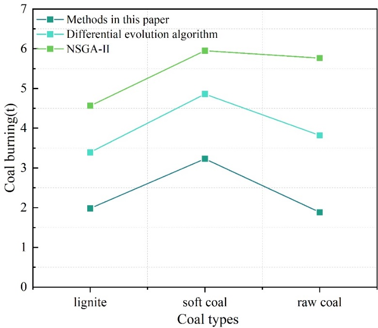
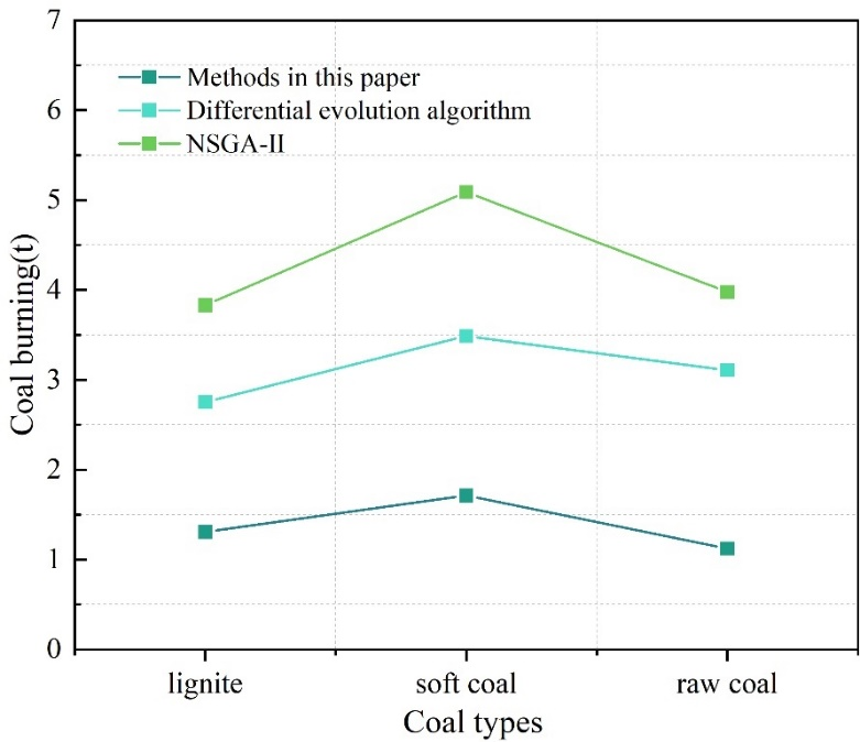
To verify the effectiveness of the method described in this paper in reducing energy consumption, the coal consumption required to produce CO\({}_{2}\) under hot start and cold start conditions was calculated separately for brown coal, bituminous coal, and raw coal. Each experiment was conducted five times, and the average value of the calculated results was obtained. By comparing the data, the ability of each algorithm to reduce energy consumption was determined. The experimental results for raw coal consumption under hot start and cold start conditions are shown in Figures 1 and 2, respectively. The results show that, when using the three types of coal, the industrial furnace’s CO\({}_{2}\) production capacity during cold start-up and hot start-up both achieve the lowest raw coal consumption using the method proposed in this paper. Therefore, the method proposed in this paper can effectively reduce energy consumption. As power plants demand lower raw material costs, the application effects of the differential evolution algorithm and NSGA-II method cannot achieve the optimal solution for reducing energy consumption, thereby proving the superior application effectiveness of the method proposed in this paper.
To determine the pollutant emissions generated by industrial furnace combustion under different algorithms, three methods were used to calculate the pollutant emissions produced by burning brown coal in industrial furnaces at different coal feed rates. The pollutant emissions are shown in Table 3. It can be seen that the method proposed in this paper results in the lowest pollutant emissions, while the other two methods yield higher emissions. This is because the method proposed in this paper optimizes the ratio of coal powder to air supply during the combustion process, thereby improving the combustion efficiency of the industrial furnace. Additionally, during the production process, the algorithm proposed in this paper optimizes the parameters of various variables in the combustion process of the industrial furnace. In summary, the method proposed in this paper demonstrates a higher ability to reduce pollutant emissions.
| Method | Coal types | Group 1 | Group 2 | Group 3 | Group 4 | Group 5 |
| Methods in this paper | Lignite | 60.36 | 58.62 | 56.68 | 58.9 | 61.13 |
| Soft coal | 66.04 | 68.47 | 61.62 | 62.65 | 63.28 | |
| Raw coal | 54.34 | 53.58 | 51.94 | 54.98 | 55.02 | |
| Differential evolution algorithm | Lignite | 86.98 | 87.86 | 87.94 | 88.73 | 89.92 |
| Soft coal | 92.32 | 91.82 | 92.27 | 92.12 | 92.85 | |
| Raw coal | 84.36 | 86.83 | 86.71 | 89.12 | 85.38 | |
| NSGA-II | Lignite | 114.84 | 113.75 | 112.73 | 113.56 | 113.49 |
| Soft coal | 105.51 | 104.01 | 103.63 | 106.34 | 107.3 | |
| Raw coal | 101.4 | 98.44 | 102.21 | 99.23 | 98.23 |
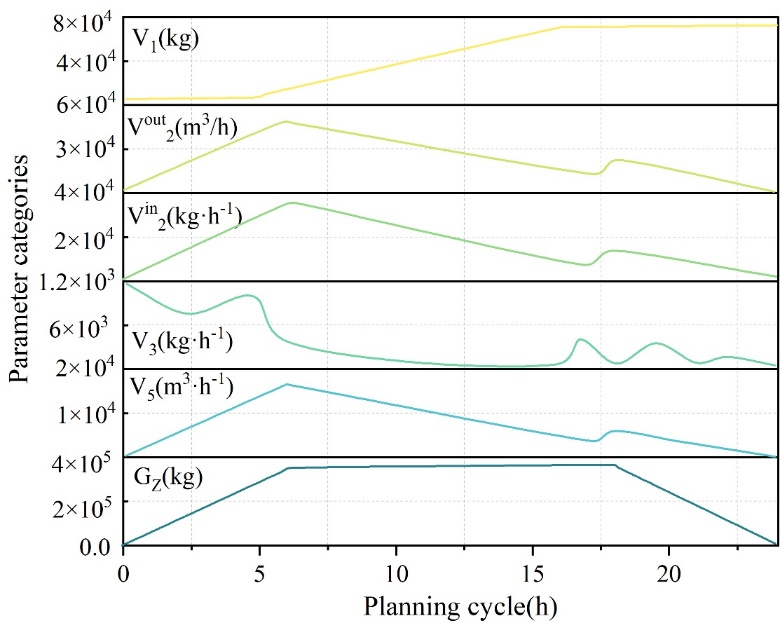
To verify the feasibility and rationality of the model, assume that the total input of raw materials is 400 tons of limestone, the production cycle is 23 hours, and the objective is to minimize fuel consumption. The mass of CO\({}_{2}\) gas in the gas holder is \(V_{1,t}\), CO\({}_{2}\) inlet flow rate to the lime kiln \(V_{2,1}^{in}\), CO\({}_{2}\) outlet flow rate from the lime kiln \(V_{2,1}^{out}\), CO\({}_{2}\) recovery rate \(V_{3,t}\), gas inlet flow rate to the heating furnace \(V_{4,t}\), and lime stone mass inside the furnace \(G_{z}\).
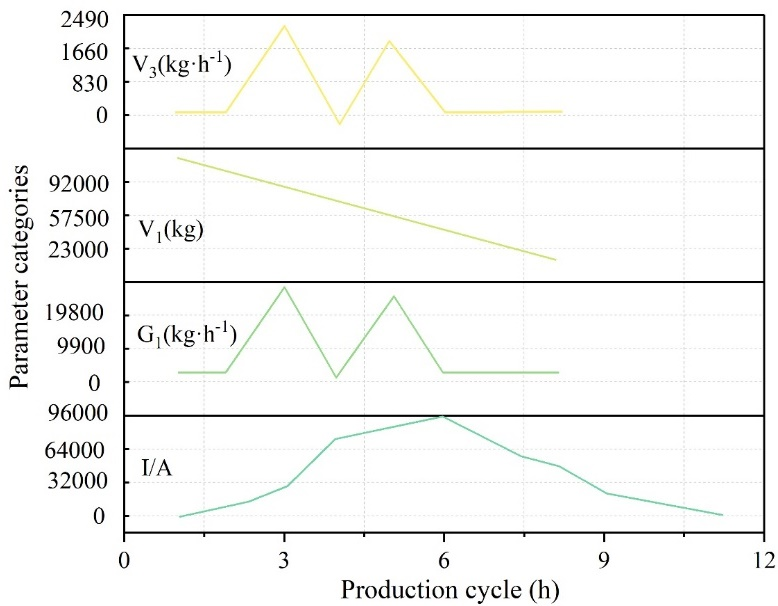
The overall scheduling results for the system are shown in Figure 3. During cycles 1 to 6, the lime kiln is in the charging phase, during which the total mass of limestone inside the kiln continuously increases until it reaches the target discharge quantity of 400 tons. According to the principles of energy conservation and mass conservation, the flow rate of hot CO\({}_{2}\) entering and exiting the kiln continuously increases to meet the gradually increasing heat load from calcium carbonate decomposition inside the kiln. Similarly, the amount of fuel required for the heating furnace to maintain the system’s operation also increases accordingly. Due to the limited CO\({}_{2}\) generated during the initial operation phase, the CO\({}_{2}\) mass in the gas holder remains stable to ensure the system’s normal operation. From cycles 7 to 17, the lime kiln is in the saturation phase, meaning that no additional calcium carbonate raw material is added to the kiln during this phase, and the thermal load inside the kiln gradually decreases from its peak. From cycles 18 to 23, the lime kiln is in the discharge phase. As calcium oxide products continue to flow out, the calcination reaction of calcium carbonate inside the kiln nears completion, resulting in a further reduction in the required amount of hot CO\({}_{2}\), and consequently, the fuel required for the lime kiln also decreases accordingly.
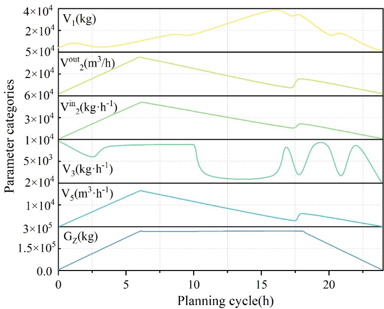
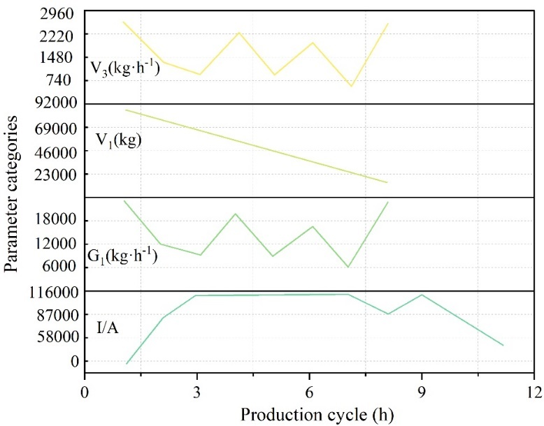
When the optimization objective is to minimize the recovery volume, the optimized overall scheduling plan results are shown in Figure 4. When the objective is to maximize CO\({}_{2}\) recovery, the gas mass in the gas holder is significantly reduced compared to the results in Figure 3, as this reduction is transferred to the CO\({}_{2}\) recovery process.
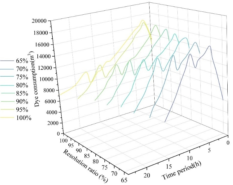
This section calculates the optimal production scheduling schemes obtained by the algorithm at target limestone decomposition rates of 65%, 70%, 75%, 80%, 85%, 90%, 95%, and 100%, and compares the differences in fuel consumption required at these decomposition rates. The system fuel allocation schemes under different decomposition rates are shown in Figure 5. The fuel input quantities corresponding to different decomposition rates are basically the same in the first six cycles. Starting from the seventh cycle, gradual differentiation begins to occur. The higher the decomposition rate, the longer the calcium carbonate remains in the furnace, resulting in a flatter decline in fuel consumption and higher overall energy consumption. When calcining 3.6\(\mathrm{\times}\)10\(^5\) kg of limestone, with a decomposition rate of 65%, the total production cycle is 5 hours, corresponding to a total fuel consumption of 14,593.77 m³ of gas, with a unit fuel consumption of 3,583.67 kJ/kg; When the decomposition rate is set to 100%, the total production cycle is 24 hours, corresponding to a total fuel consumption of 17,007.94 m\(^3\), with the unit fuel consumption increasing to 4,572.82 kJ/kg. As the limestone decomposition rate increases from 65% to 100%, the unit fuel consumption per product increases by 41.91 kJ/kg, 39.37%, 26.22 kJ/kg, 27.83 kJ/kg, 19.43 kJ/kg, and 28.34 kJ/kg for each 5% increase, with the overall trend of fuel consumption increase decreasing.
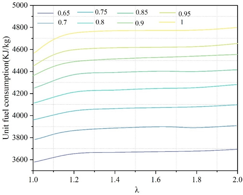
Based on the above analysis, the ratio of the total limestone feed rate to the rated capacity of the lime kiln is defined as \(\lambda\). A higher \(\lambda\) value indicates a greater extent to which the target calcium carbonate production exceeds the rated capacity of the kiln. The changes in fuel consumption per unit under different \(\lambda\) conditions are shown in Figure 6. It can be observed that, under the same decomposition rate, as \(\lambda\) gradually increases from 1 to 2, the unit fuel consumption per product of the system shows a slow increase. Further analysis reveals that, at a decomposition rate of 65%, when \(\lambda\) is 1, the system’s unit fuel consumption is 3,583.67 kJ/kg, and when \(\lambda\) is 2, the system’s unit fuel consumption increases to 3,696.41 kJ/kg, representing a growth rate of 3.15%. When \(\lambda\) is 1, if the decomposition rate is increased from 65% to 100%, the unit fuel consumption increases from 3,583.67 kJ/kg to 4,572.82 kJ/kg, with a growth rate of 27.6%. This indicates that, compared to \(\lambda\), the decomposition rate has a greater impact on operational energy consumption. Therefore, in actual production decision-making, companies should make comprehensive decisions based on their own needs, balancing product quality (decomposition rate) and operational energy consumption costs.
1) Overall system dispatch results with the goal of minimizing unit energy consumption
The unit energy consumption for this production plan is 3583.67 kWh·t-1. During any t-period within the entire production cycle, the mass flow rate of pyrolysis furnace gas in the gas storage tank is \(V_{1,t}\), the outlet flow rate from the preheated pyrolysis furnace is \(V_{2,t}\), and the mass flow rate entering the preheated pyrolysis furnace is \(V_{3,t}\). the mass flow rate of pyrolysis furnace gas used for resource recovery is \(V_{4,t}\), the current supplied to the mineral electric furnace is \(I_{t}\), and the mass flow rate of cold pellets supplied is \(G_{1,t}\).
The overall scheduling results of the system with the objective of minimizing specific power consumption are shown in Figure 7. During cycles 1 to 8, the pyrolysis furnace is in the feeding, pellet preheating pyrolysis, and discharging stages, while the mineral electric furnace is in the discharging stage. Due to the limited amount of furnace gas generated in the pyrolysis furnace during the initial operation phase, the furnace gas in the gas storage tank needs to be continuously consumed to maintain stable calcium carbide production. Correspondingly, during cycles 6 to 11, as the feed rate in the mineral furnace has peaked and is rapidly decreasing, the furnace no longer requires a higher current to maintain high power.
) Overall system scheduling results with maximum output as the objective
At the same time, for the production scheduling model of the mixed preheated pelletized ore hot blast stove, this chapter solves the model with maximum calcium carbide output as the objective. The overall system scheduling results with maximum output as the objective are shown in Figure 8. The scheduling scheme corresponding to the objective of maximizing production volume has an average feed rate in the first and second cycles that far exceeds that of the production scheme targeting minimum unit power consumption. When considering all production cycles, its average feed rate is also greater than the latter. Therefore, its power supply reaches a peak in the third cycle and remains at a high level thereafter, only decreasing after the end of feed supply in the eighth cycle. Therefore, in actual production, enterprises should pay attention to the balance between unit electricity consumption and calcium carbide production when formulating production plans. It is recommended to use multi-objective optimization methods to address this issue.
This paper proposes a fuzzy neural network control model for multi-variable systems by combining the advantages of fuzzy control and artificial neural networks, providing decision-making and control for improving the combustion efficiency of industrial furnaces.
The fuzzy neural network control model for multi-variable systems proposed in this paper can improve the combustion efficiency of industrial furnaces, reduce the concentration of emissions, and decrease energy consumption, thereby achieving optimized management and control of the combustion process in industrial furnaces. When the fuel decomposition rate increases from 78% to 100%, the growth rate of unit fuel consumption decreases, indicating the model’s effective application. Additionally, in actual production, this paper recommends that enterprises consider the balance between unit electricity consumption and calcium carbide production when formulating production plans.