With the continuous advancement of manufacturing technology, CNC machine tools have become indispensable equipment in modern manufacturing [1]. During CNC turning processes, tool wear is an inevitable phenomenon. Tools gradually degrade and wear due to friction with the workpiece surface, leading to reduced cutting efficiency and degraded processing quality [2– 4]. Additionally, tool wear not only increases material and energy consumption but may also cause production interruptions and additional maintenance costs [5, 6]. Therefore, as the core processing component of CNC machine tools, precise monitoring of tool wear status not only ensures the safe operation of machining centers and improves production efficiency but also enhances the quality of processed parts [7– 9]. If tool wear is excessive or not detected in a timely manner, it can lead to reduced surface quality of the workpiece, decreased processing accuracy, and even production accidents, resulting in economic losses [10– 12]. Traditional tool wear monitoring methods, such as relying on the operator’s experience or specialized instruments for measurement, are not only time-consuming and labor-intensive but often fail to meet the demands of high-quality and efficient processing [13, 14]. Methods relying on experience have inherent limitations due to their lag and subjectivity, which can lead to inconsistent judgments due to individual differences, thereby affecting the accuracy of tool wear monitoring [15, 16]. Direct monitoring methods using specialized instruments, on the other hand, require interrupting the production process, leading to reduced production efficiency [17]. In this context, the limitations of traditional monitoring methods become particularly evident. With the development of smart manufacturing, there is an increasing demand for more efficient and intelligent tool wear monitoring methods. A method capable of continuously and online monitoring tool status is needed to ensure the continuity of machining and the quality of parts [18– 21].
Initially, scholars proposed tool monitoring methods based on physical models, which rely on analyzing tool wear mechanisms and describing tool wear processes through physical relationship models. For example, Li [22] found that tool wear results from contact and relative sliding between the cutting tool and the chip, and thus employed the finite element method to explore the evolution of tool wear and predict tool life. Ramírez et al. [23] designed a finite element analysis method for tool wear based on dimensional analysis and metal cutting, establishing a numerical model of cutting to enable prediction of tool surface pitting wear based on local parameter variables. Nooraie et al. [24] focused on the geometric shape of worn tools and changes in the inclination angle of the wear region, combining finite element simulation with response surface methods to construct a wear rate equation, achieving effective tool wear condition monitoring. Han et al. [25] found that metal cutting is often accompanied by temperature changes. They proposed using thermal radiation spectroscopy to measure tool temperature in real-time during cutting and developed a tool wear state identification model based on cutting temperature, which holds significant application potential in CNC machining. Han et al. [26] utilized a fiber-optic dual-color high-temperature meter to obtain real-time temperature data of the cutting edge during turning and established a mapping model between temperature changes and tool wear. However, tool monitoring methods based on physical models only consider the dominant factors related to tool wear, making it difficult to establish accurate physical models and resulting in large prediction errors. In addition, environmental interference and individual differences between tools and workpieces also reduce the accuracy of tool monitoring methods based on physical models.
With the development of artificial intelligence technology, data-driven tool wear monitoring methods based on machine learning have also attracted the attention of researchers. Cheng et al. [27] developed a novel tool condition prediction model based on feature normalization, attention mechanisms, and deep learning algorithms, enabling short-term and long-term predictions of tool wear states under different cutting parameter combinations. Munaro et al. [28] investigated the application of artificial intelligence technology in tool wear monitoring, proposing and validating the feasibility of an artificial intelligence system predicting tool wear based on tool behavior. Li et al. [29] utilized extended principal component analysis to process and analyze multi-channel audio signals during machine tool processing, constructing an intelligent classification model capable of distinguishing tool wear states at different stages. Gouarir et al. [30] introduced an adaptive control (AC) system integrating machine learning models with force sensor data feedback, which can accurately determine tool wear states and propose processing decisions to extend tool life. de Farias et al. [31] found that combining machine learning methods with data-driven methods significantly improves the prediction accuracy of tool wear states. They proposed applying optimal linear associative memory neural networks and self-organizing deep learning models to industrial machine tool processing, providing valuable recommendations for tool replacement and maintenance. Although data-driven tool wear monitoring methods can accurately assess tool health status, relying solely on feature extraction methods to determine tool status lacks generalizability of results.
Tool status monitoring methods based on data and physics (mechanism) hybrid models combine the advantages of physics-driven models and data-driven models to achieve monitoring models with higher monitoring accuracy and robustness. Zhang et al. [32] considered the inaccuracy of physics-based tool wear models in complex machining environments and proposed establishing a deep mapping relationship between signal data and tool wear to achieve accurate monitoring of tool wear status. Goodall et al. [33] evaluated the power consumption of CNC machines and related parameters of tool milling, and after extensive repetitive testing, ultimately developed a cyber-physical system that accurately reflects tool condition monitoring information. Yuan et al. [34] applied a model-driven cyber-physical system based on the Extended Kalman Filter (EKF) method to machine tool condition monitoring, overcoming the limitations of traditional physical models by calibrating the constructed empirical model using online measurement data. Hanachi et al. [35] proposed using regularized particle filtering technology to perform numerical inference on monitoring data based on physical principles and sensors, thereby updating tool wear state predictions in CNC machine tools and significantly reducing monitoring result errors. Zhu et al. [36] established a physics-based hidden Markov model (PI-HMM), which can constrain the division of hidden states on one hand and incorporate expanded training datasets into the output model on the other, thereby effectively improving the recognition accuracy of tool wear monitoring. Wang et al. [37] used particle filter technology to fuse the results of physical model-based and data-driven tool wear condition monitoring, achieving higher accuracy and better physical consistency compared to a single model. Ma et al. [38] proposed a hybrid-driven probabilistic state space model to improve the accuracy and robustness of tool wear monitoring, utilizing Gaussian processes to deeply mine measurement data and incorporate it into the physical model, playing a crucial role in estimating tool wear conditions . Lee et al. [39] monitored temperature changes at the peak of cutting tools by establishing a heat transfer coefficient solution model in the far field and an artificial neural network training model in the near field, providing support for monitoring the wear status of CNC machine tool blades. It is evident that the aforementioned research methods effectively combine the advantages of physical models and data-driven models, enhancing the interpretability and generalizability of the models.
The article provides an in-depth analysis of the mechanisms underlying tool wear, categorizes the wear stages, and utilizes the PHM and NASA public datasets as the primary data sources for milling experiments. It also introduces and analyzes the monitoring data from both datasets. Based on a deep residual network, the noise interference in tool wear signals is reduced by calculating a soft threshold function. DropBlock regularization technology is introduced to regularize the feature maps of the convolutional layers, enhancing the model’s ability to resist interference. The optimized deep residual contraction network model is trained and evaluated for tool wear monitoring, with an analysis of the model’s effectiveness and tool wear recognition performance.
Tool wear occurs as a result of the cutting forces generated by the contact between the tool, workpiece, and chips. In most cases, tool wear is a normal phenomenon, while the remaining individual cases of wear are typically abnormal. To better monitor the condition of tool wear, it is essential to understand the mechanisms and processes involved in tool wear.
During machining processes, mechanical forces are at work, accompanied by heat generation and corresponding chemical reactions. These are the primary causes of tool wear, which can be attributed to the following types of factors.
1) Abrasive wear
When high-speed machining begins, the surface layer of the workpiece is subjected to intense friction and impact, causing plastic deformation and micro-cracks in the surface layer, thereby forming grinding grooves.
2) Diffusion wear
Under the intense pressure of interacting forces, the constituent elements of the processed material undergo mutual fusion, causing changes in their respective compositions and structures.
3) Oxidation wear
As temperature rises, oxidation occurs on the tool surface, forming softer oxides. Wear is caused by friction between chips, which is known as oxidation wear. Oxidation is a non-cutting phenomenon induced by high temperatures.
4) Adhesive wear
Under specific pressure and temperature conditions, the cutting portion of the tool comes into contact with the chip and undergoes friction. Adsorption occurs between the molecules of the material, leading to adhesive wear.
5) Cold welding wear
During the cutting process, high pressure and intense friction occur between the workpiece, chip, and front and rear tool surfaces, resulting in cold welding.
Based on the differences in the machining process and the extent of tool wear, the tool wear process is divided into three stages: initial wear, normal wear, and severe wear.
1) Initial wear
When machining first begins, the tool is relatively new, and its cutting edge is extremely sharp. The sharp cutting edge results in a small contact area between the tool and the workpiece, causing significant stress concentration at the tool tip, thereby accelerating the surface grinding speed during the machining process.
2) Normal wear
During the normal wear stage, the contact area between the tool and the workpiece, as well as the contact stress between them, is highly stable, characterized by surface contact and relatively low stress.
3) Severe wear
The severe wear stage is the most critical phase of wear, particularly toward the latter part of this stage, which significantly impacts the tool’s cutting performance. At this stage, the surface structure of the tool no longer meets the machining accuracy requirements, and the tool’s performance has significantly deteriorated compared to the previous stage.
Tool life is influenced by various factors, including differences in cutting processes and changes in workpiece and tool materials. Typically, tool life is described by Taylor’s formula, which can be expressed as: \[\label{GrindEQ__1_} V_{c} Tn\times a_{p} xv_{f} y=C, \tag{1}\] where,\(V_{c}\) represents the cutting speed, \(T\) represents the tool life, \(a_{p}\) represents the back cutting depth, and \(v_{f}\) represents the feed rate. \(x\) and \(y\) are determined experimentally. \(n\) and \(C\) are constants representing the characteristics of the tool material, workpiece, and feed rate.
In this paper, tool milling data collected from the High-Speed CNC Machine Tool Tool Health Prediction Competition organized by the Predictive and Health Management (PHM) Association was selected as one of the datasets for this study.
By repeating the full life cycle experiment 10 times under the same machining conditions, relevant signal data from 5 milling cutters were collected across the 10 experiments. In three of these measurements, wear values of the rear surfaces of the three cutting edges of the milling cutters were also collected. The PHM dataset used in this study consists of these three datasets, which include wear values and corresponding tool monitoring signal data.
The signal types collected in the milling cutter wear dataset include milling force signals, vibration signals in the X, Y, and Z directions of the three coordinate axes, and the root mean square (RMS) values of acoustic emission (AE) signals, totaling seven types of data.
To validate the proposed model’s ability to predict tool wear under varying operating conditions, a publicly available NASA dataset was also incorporated. The experiments conducted using this dataset involved milling operations performed on a Matsuura machining center, with different cutting parameters and machining conditions employed throughout the experiments. Signal acquisition utilized multiple sensors to collect vibration and acoustic emission signals from the worktable and spindle, as well as current signals from the DC spindle motor and AC spindle motor, with a sampling frequency of 100 kHz.
One of the most notable features of deep learning is the “depth” of its network layers. By stacking deep layers, it achieves higher accuracy in image processing tasks, enabling the system to possess sharp image and speech recognition capabilities [40, 41]. A simple neural network consists of an input layer, an output layer, and hidden layers. The neural network first calculates the output result through forward propagation i(n)-h(n)-o(n), then compares it with the sample to determine the error, and finally adjusts the gradient of the weights in the backward direction. The process of training the neural network involves continuously adjusting the parameter matrix. During backpropagation through the hidden layer, the neural network continuously updates the parameter matrix. However, as the number of network layers increases, the gradient of the parameter matrix gradually diminishes, and gradient decay becomes more severe, leading to the network being unable to perform backpropagation weight adjustments.
A deep residual network (DRN) is a type of deep convolutional network [42]. Given a network input \(x\), we want the output to be \(H(x)=F(x)+x\), so the network only needs to learn the residual \(F(x)\) between \(H(x)\) and \(x\). By directly adding an identity connection to the original network, fitting \(H(x)\) and the residual function \(F(x)\) is equivalent, and the original function becomes \(H(x)\), thereby passing the identity mapping of \(x\) to the output.
The key to incorporating attention mechanisms into deep learning networks is to enable the network to adaptively focus on the areas that require attention. Attention mechanisms can be divided into two aspects: channel and spatial. Among these, the SENet algorithm and ECA algorithm are based on channel attention mechanisms.
This paper takes the SENet algorithm as the core attention mechanism, which is an algorithm that applies channel attention mechanisms [43]. Channel weights are obtained through a convolutional neural network, and a “recalculate feature weights” strategy is adopted to learn the importance of each feature channel and adjust the weight parameters, thereby re-calibrating the features in the channel dimension. This method involves a high computational load but enables the network to learn the correlations between channels. Inputting the channel attention map output by SENet into the next-level network model can improve the model’s accuracy. The specific process is as follows:
Input a feature map of size \(C\times H\times W\), first compress the feature map using global average pooling to obtain a feature map of size \(1\times 1\times C\), followed by two fully connected layers for nonlinear transformation. Finally, the values are fixed within the 0–1 range via the Sigmoid function, and the resulting weights are multiplied by the corresponding input feature vector of the channel, thereby achieving “feature recalibration” on the channel attention level.
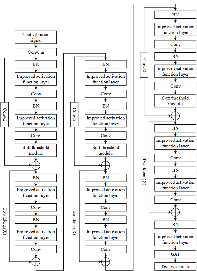
This paper focuses on tool wear monitoring in precision machining of CNC machine tools. Based on the key technologies described above, an improved residual contraction network structure is designed, as shown in Figure 1. The preprocessed tool vibration monitoring signals are used as input, and multiple improved residual contraction modules are used for feature extraction. Finally, after passing through the GAP layer, the monitoring results of the tool wear status are output.
The soft threshold function is a key step used in many signal denoising methods. The calculation method for soft thresholding is as follows: \[\label{GrindEQ__2_} y=\left\{\begin{array}{ll} {x-\tau } & {x>\tau }, \\ {0} & {-\tau \le x\le \tau } ,\\ {x+\tau } & {x<-\tau }. \end{array}\right. \tag{2}\]
In the equation, \(x\) represents the input signal value, \(y\) represents the output after soft thresholding, and \(\tau\) is the set threshold, i.e., a positive parameter. Unlike the ReLU activation function, which directly sets all negative features to zero, soft thresholding sets features close to zero to zero, thereby retaining useful negative features without affecting the actual recognition performance. During soft thresholding, the inverse of the input corresponding to the output is either 1 or 0, which avoids the issues of gradient explosion and gradient vanishing when applied to neural networks. Its derivative is as follows: \[\label{GrindEQ__3_} \frac{\partial y}{\partial x} =\left\{\begin{array}{ll} {1} & {x>\tau } ,\\ {0} & {-\tau \le x\le \tau }, \\ {1} & {x<-\tau }. \end{array}\right. \tag{3}\]
Deep Residual Contraction Networks (DRCNs) are a variant of residual networks designed for noisy signals, with a basic structure similar to that of the basic modules of residual networks. The key improvement lies in the use of neural networks to autonomously learn and generate thresholds, thereby achieving soft thresholding of features.
Batch normalization (BN) and ReLU are used as batch normalization processing and activation functions, respectively, while Conv represents the convolution layer. By introducing weights generated through autonomous learning as thresholds on top of the residual module, soft thresholding of features is achieved, thereby reducing the impact of noise. To ensure that the thresholds are positive and not excessively large, the results of global average pooling are first subjected to absolute value processing to ensure positive values, and then multiplied by the learned weights to obtain the thresholds, thereby ensuring that the generated thresholds do not become excessively large.
This study addresses the problem of difficulty in monitoring tool wear status in noisy environments by proposing an improved activation function layer that fully utilizes monitoring signals and anti-interference capabilities to enhance the tool wear status recognition performance of neural network models.
Currently, commonly used activation functions in neural networks include ReLU and Sigmoid. The calculation process of the Sigmoid activation function is as follows: \[\label{GrindEQ__4_} y_{sigmoid} =\frac{1}{1+e^{-x_{xigmoid} } } . \tag{4}\]
In the formula, \(x_{sigmoid}\) represents the input of the Sigmoid activation function, and \(y_{sigmoid}\) represents the output calculated by the Sigmoid activation function.
ReLU is currently the most commonly used activation function in neural networks. Its calculation process is as follows: \[\label{GrindEQ__5_} y_{ReLU} =\left\{\begin{array}{ll} {x_{ReLU} } & {x_{ReLU} >0}, \\ {\quad 0} & {x_{ReLU} \le 0}. \end{array}\right. \tag{5}\]
In the equation, \(x_{ReLU}\) represents the input of the ReLU activation function, and \(y_{ReLU}\) represents the output after calculation by the ReLU activation function.
During the monitoring of tool wear status, the original vibration monitoring signals often contain a large number of negative values. If the ReLU activation function is used in the tool wear status recognition model, the negative values in the vibration monitoring signals will be discarded, failing to fully utilize the signal characteristics and significantly weakening the neural network model’s performance in recognizing tool wear status. To address this issue, an activation function with negative outputs, SiLU, is employed. Its calculation process is as follows: \[\label{GrindEQ__6_} y_{SILU} =x\cdot Sigmoid(x) . \tag{6}\]
This activation function is based on the Sigmoid activation function, with the output obtained by multiplying the input. This approach does not completely eliminate negative output values in tool vibration monitoring signals, thereby fully utilizing the vibration monitoring signals while preventing gradient dispersion.
In the current tool wear state recognition neural network model, the anti-interference capability of the model is enhanced in most cases by using a manually set Dropout regularization rate in the fully connected layer, which reduces the correlation between neurons as a form of data augmentation to mitigate overfitting.
To address the issue of Dropout being ineffective for convolutional layers, DropBlock regularization technology was introduced to regularize feature maps in convolutional layers. This method no longer involves dropping individual neurons but instead deletes a continuous region of the feature map, thereby reducing the risk of overfitting and enhancing the model’s resistance to interference. The calculation process for DropBlock is as follows: \[\label{GrindEQ__7_} \gamma =\frac{1-keep\_ prob}{block\_ size^{2} } \frac{feat\_ size^{2} }{(feat\_ size-block\_ size+1)^{2} }, \tag{7}\] keep_prob is the probability of a neuron being disabled in traditional Dropout, feat_size represents the size of the feature map, and \(\gamma\) represents the number of features to be deleted.
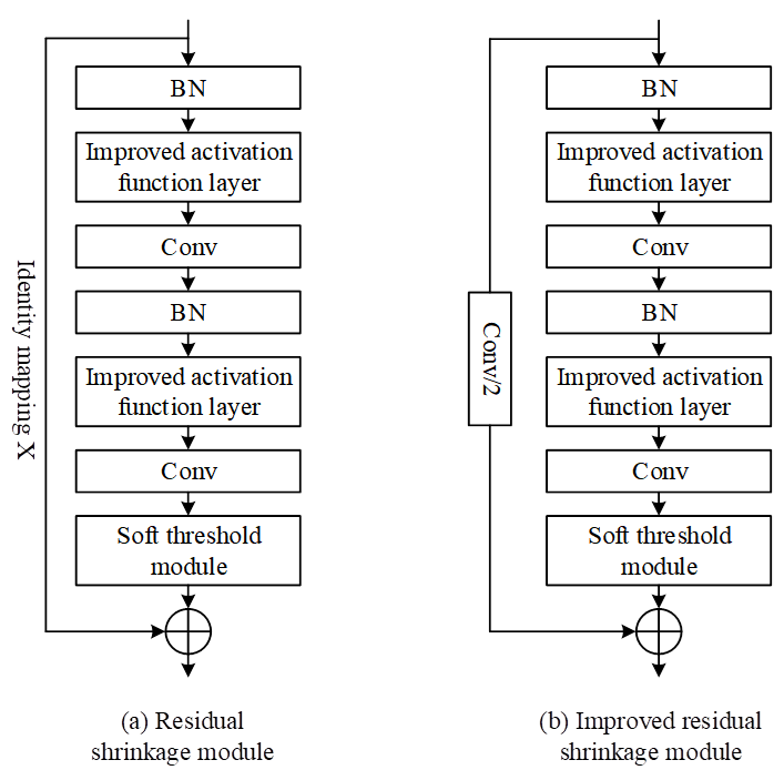
The improved residual contraction module is shown in Figure 2, where BN denotes batch normalization, Conv represents the convolution layer, and X represents the input. Compared with the original module, the improved residual contraction module replaces the ReLU activation function with the improved activation function layer proposed in this paper.
To validate the effectiveness of the tool wear monitoring model designed in this paper, the model was trained and tested. The Dropout parameter was set to 0.2, and the number of iterations was set to 200. The monitoring accuracy and loss function iteration process of the model during the training process are shown in Figure 3.
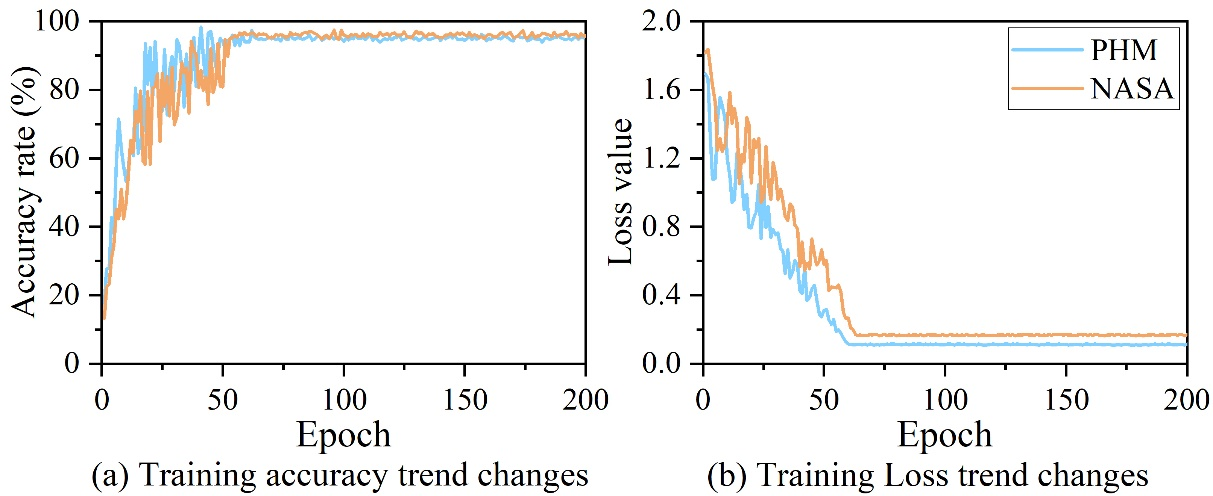
As shown in the figure, on the PHM and NASA datasets, the model becomes more stable as the number of iterations increases, with significant fluctuations in loss and accuracy during the first 25 iterations. Specifically, when the model reaches approximately 60 epochs, the monitoring accuracy for tool wear on both datasets stabilizes above 95%. For the loss function, the model converged after 60–65 iterations, achieving loss function values of 0.12 and 0.17 on the PHM and NASA datasets, respectively. Compared to previous studies, the accuracy of the proposed model is approximately 3%–10% higher than that of traditional models, and its training and prediction performance outperforms most reported models, demonstrating the feasibility and superiority of the proposed model.
To further analyze the performance of the tool wear monitoring model based on the improved deep residual contraction network in this paper, convolutional neural networks (CNN), long short-term memory neural networks (LSTM), and support vector machine models (SVM) were selected as comparison models. The recognition accuracy rates of the four models for three different tool wear states in the test set were calculated separately.
The recognition accuracy rates of different models for different wear states are shown in Table 1. During the normal wear stage, the recognition accuracy rates of all four models were higher than those in the other two wear stages, primarily because the normal wear stage had the largest number of samples, making the models more stable in this stage. Across different wear stages, among the three comparison models, the CNN model performed best, while the LSTM model and SVM model performed similarly. However, they were slightly inferior to the model proposed in this paper, with the CNN model having an accuracy rate 3%–5% lower. This indicates that introducing an attention mechanism while improving the network’s key modules can effectively allocate feature weights, thereby aiding in the accurate identification of tool wear.
| Type | Accuracy rate (%) | |||
| CNN | LSTM | SVM | Ours | |
| Initial wear | 93.15 | 91.53 | 90.54 | 97.29 |
| Normal wear | 94.51 | 93.19 | 91.67 | 99.13 |
| Severe wear | 92.23 | 89.24 | 88.42 | 95.39 |
To more accurately evaluate the overall performance of the proposed deep learning tool wear monitoring model, different evaluation parameters were calculated for the four models, including sensitivity, specificity, precision, and F1 score.
| Type | Model | Sensitivity (%) | Specificity (%) | Recall (%) | F1 (%) |
|---|---|---|---|---|---|
| Initial wear | CNN | 93.69 | 93.02 | 91.55 | 94.01 |
| LSTM | 90.91 | 92.47 | 91.8 | 92.36 | |
| SVM | 91.45 | 91.2 | 90.48 | 93.38 | |
| Ours | 96.83 | 98.42 | 96.97 | 97.64 | |
| Normal wear | CNN | 94.93 | 90.33 | 93.05 | 93.26 |
| LSTM | 93.67 | 91.79 | 90.3 | 90.12 | |
| SVM | 92.05 | 91.59 | 92.22 | 93.98 | |
| Ours | 99.62 | 99.76 | 98.7 | 96.49 | |
| Severe wear | CNN | 93.14 | 94.99 | 94.14 | 91.95 |
| LSTM | 92.07 | 91.75 | 94.43 | 92.42 | |
| SVM | 92.01 | 90.84 | 92.32 | 93.87 | |
| Ours | 98.76 | 98.15 | 98.26 | 98.23 |
The performance comparison results of the three tool wear monitoring models are shown in Table 2. As shown in the table, the sensitivity of all three models is highest during the normal wear stage, indicating that the false negative rate is lowest in this stage. The sensitivity of the proposed model is higher than that of the comparison models in all stages. Additionally, the specificity of the comparison models fluctuates significantly across different wear stages, resulting in lower reliability and model instability. In contrast, the specificity of the proposed model remains above 98% throughout. Furthermore, in terms of precision and F1 scores, the proposed model achieved the highest values across different wear states, with the F1 score reaching a maximum of 98.23% during severe wear. This indicates that the model demonstrates the best overall performance when monitoring tool condition during the severe wear stage. Based on the experimental data, the proposed model’s evaluation parameters outperform those of the comparison models, exhibiting extremely high reliability and making it highly suitable for tool wear monitoring.
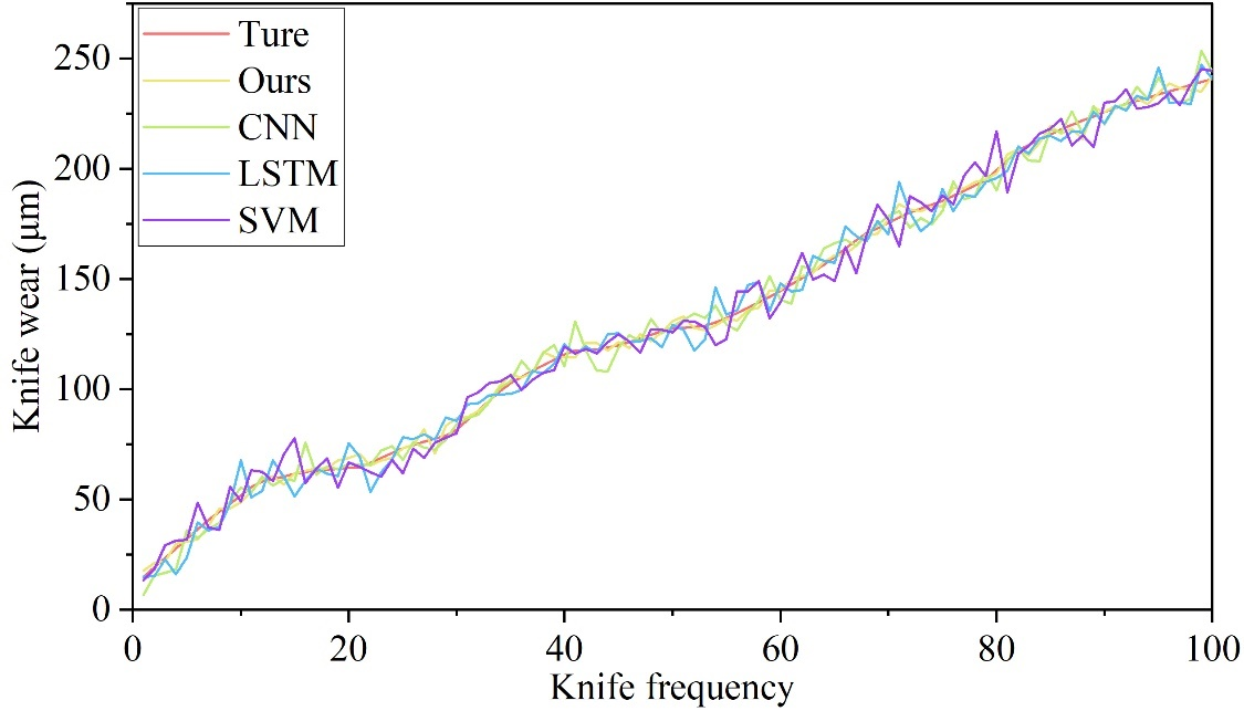
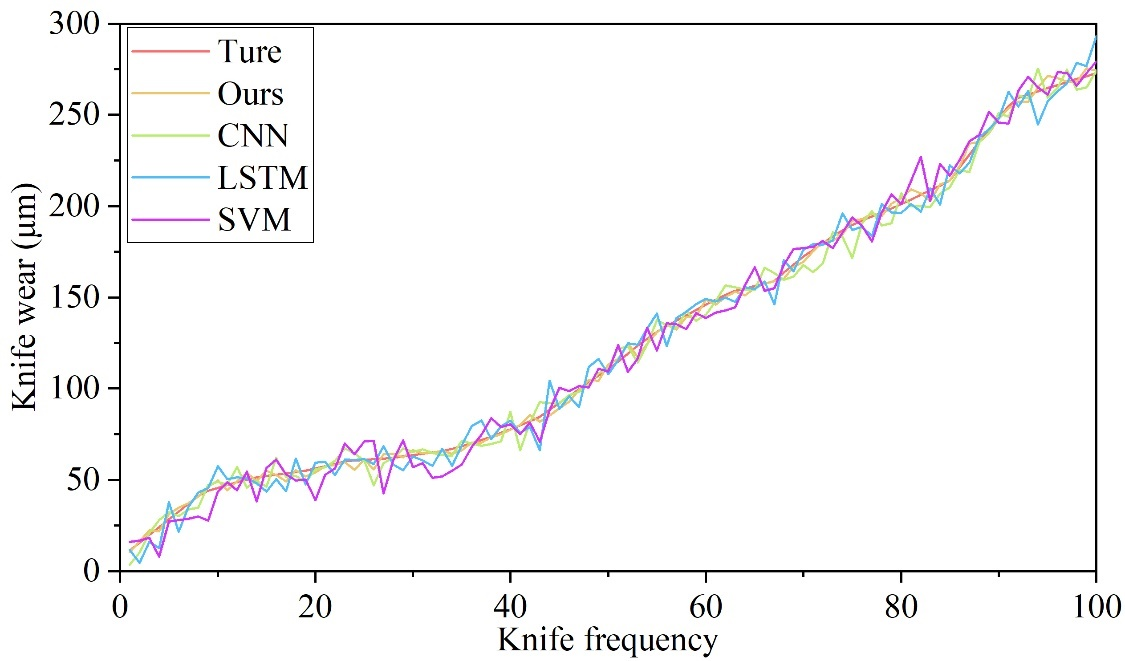
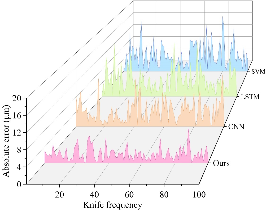
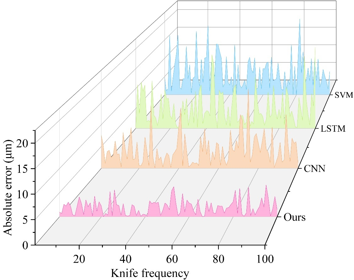
To validate the effectiveness of the tool wear monitoring model proposed in this paper, we tested and analyzed the performance of the model by comparing the prediction accuracy of four different models in the task of online monitoring and early warning of tool wear in CNC machine tools. Figures 4 and 5 show the monitoring results of rear face wear for different models on the PHM and NASA datasets, respectively. As can be seen from the figures, the prediction curves of these methods generally show an upward trend, consistent with the characteristic of tool wear accumulating over time. However, compared with the method proposed in this paper, the other methods exhibit significant fluctuations. Additionally, Figures 6 and 7 show the absolute identification errors of different models in detecting rear tool face wear on the PHM and NASA datasets, respectively. Statistically, the absolute error in identifying tool wear throughout the entire wear period for the proposed model ranges from 0 to 8.5 \(\mu\)m, while the identification error for the comparison models can reach up to 20.7 \(\mu\)m. When tool wear reaches a certain threshold, cutting force and cutting temperature increase sharply, accelerating the rate of tool wear and increasing the difficulty of identification. The proposed model demonstrates high sensitivity in identifying tool wear throughout the entire wear period, thereby validating the superiority of the proposed method.
In order to quantitatively compare the performance of the model in this paper with that of traditional models on different datasets, the root mean square error (RMSE), mean absolute error (MAE), and coefficient of determination (\(R^{2}\)) of the monitored tool wear values and actual tool wear were calculated. The calculation methods for these three indicators are as follows: \[\label{GrindEQ__8_} RMSE=\sqrt{\frac{1}{N} \sum _{i=1}^{N}(p_{i} -y_{i} )^{2} } , \tag{8}\] \[\label{GrindEQ__9_} MAE=\frac{1}{N} \sum _{i=1}^{N}|p_{i} -y_{i} | , \tag{9}\] \[\label{GrindEQ__10_} R^{2} =1-\frac{\sum _{i}(p_{i} -y_{i} )^{2} }{\sum _{i}(\overline{y_{i} }-y_{i} )^{2} } . \tag{10}\]
In the equation, \(N\) is the total number of samples, \(p_{i}\) is the \(i\)th monitored wear value, \(y_{i}\) is the \(i\)th actual wear value, and \(\bar{y}_{i}\) is the mean of the actual wear values. Smaller RMSE and MAE values and larger \(R^{2}\) values indicate better predictive performance of the model.
Table 3 quantitatively evaluates the performance of different monitoring models based on RMSE, MAE, and R2 metrics. Comparing these results, it can be observed that the identification accuracy of the proposed model is higher than that of the comparison models on both datasets, demonstrating the positive effect of deep residual networks and attention mechanisms on tool wear monitoring. Compared to the comparison models, for example, in the PHM dataset, the RMSE and MAE of the proposed method are 13.29 and 12.15, respectively, representing a reduction of over 56% compared to the comparison methods. Additionally, regardless of the dataset, the proposed method achieves the highest R² value, with an improvement of up to 6.55 percentage points. This demonstrates that the proposed method significantly outperforms other methods in terms of overall performance and exhibits good generalization capabilities.
| Date set | Model | RMSE | MAE | R\({}^{2}\) (%) |
|---|---|---|---|---|
| PHM | Ours | 13.29 | 12.15 | 98.29 |
| CNN | 20.86 | 21.48 | 95.89 | |
| LSTM | 24.47 | 26.82 | 91.74 | |
| SVM | 23.03 | 24.24 | 93.91 | |
| NASA | Ours | 14.56 | 11.94 | 97.25 |
| CNN | 18.52 | 20.02 | 94.92 | |
| LSTM | 22.8 | 21.26 | 92.08 | |
| SVM | 21.78 | 20.59 | 90.89 |
In this study, the number of positive samples correctly identified as positive can be represented as \(TP=\{ TP_{I} ,TP_{N} ,TP_{S} \}\), and the number of positive samples incorrectly identified as other categories can be represented as \(FN=\{ FN_{I} ,FN_{N} ,FN_{S} \}\), and the number of negative samples correctly classified as positive samples can be represented as \(FP=\{ FP_{I} ,FP_{N} ,FP_{S} \}\), where the subscripts \(I,N,S\) denote the initial wear stage, normal wear stage, and severe wear stage, respectively.
Using the severe wear stage as an example, the recall rate and precision rate can be calculated as follows: \[\label{GrindEQ__11_} R_{S} =\frac{TP_{S} }{TP_{S} +FN_{S} } \times 100\% , \tag{11}\] \[\label{GrindEQ__12_} P_{S} =\frac{TP_{S} }{TP_{S} +FP_{S} } \times 100\% . \tag{12}\]
In the formula, \(w\) is the weighting factor, and \(w_{1} ,w_{2} ,w_{3}\) are set to 0.15, 0.4, and 0.45, respectively. The calculations yield the recall rates and precision rates for the three categories, denoted as \(R=\{ R_{I} ,R_{N} ,R_{S} \}\) and \(P=\{ P_{I} ,P_{N} ,P_{S} \}\), respectively. Assigning different weights to the recall and precision rates for different wear stages is referred to as RWA (Recall Weighted Average) and PWA (Precision Weighted Average). Weakening the weight of the initial wear stage and strengthening the weight of the severe wear stage, the average of the three stages is used as the final recall and precision rates for identification. RWA and PWA can be expressed as: \[\label{GrindEQ__13_} RWA=w_{1} R_{I} +w_{2} R_{N} +w_{3} R_{S} , \tag{13}\] \[\label{GrindEQ__14_} PWA=w_{1} P_{1} +w_{2} P_{N} +w_{3} P_{S} . \tag{14}\]
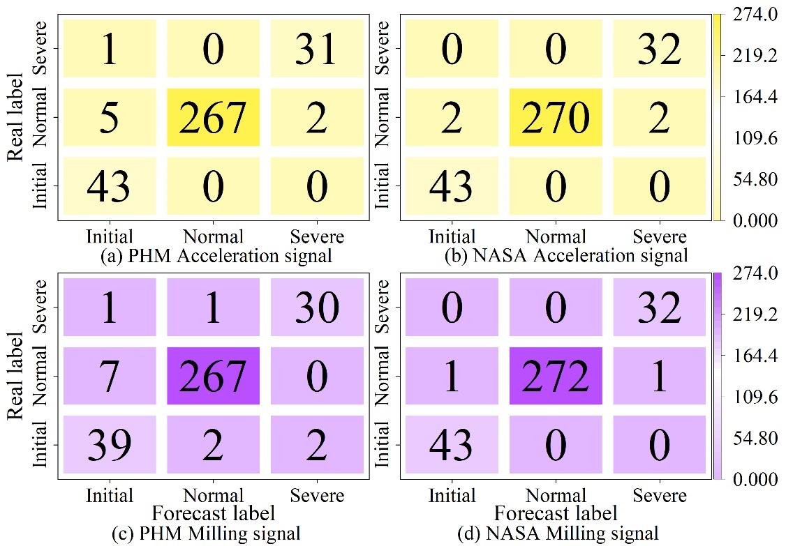
The confusion matrix is used to visually evaluate the model’s recognition results for imbalanced data categories. Figure 8 shows the tool wear state recognition results after different sensing signals are input into the model. Among them, Figures 8 (a) and (b) show the results based on acceleration signals, while Figures 8 (c) and (d) show the results based on milling force signals. It is worth noting that the model structures for both signal inputs are identical, thereby avoiding the issue of model retraining caused by sensor replacement in actual machining environments. As shown in the figure, both signals demonstrate excellent performance in identifying the severe wear stage, validating the model’s generalization capability across different sensory signals. Specifically, in Figure 8(d), the recall rate and accuracy for the severe wear stage exceed 95%, achieving very good results. The identification results based on cutting force signals are more accurate, as cutting force is more sensitive to tool wear. Notably, the number of samples incorrectly identified as the severe wear stage from other categories is nearly zero, which avoids downtime losses caused by misjudging the tool change timing in actual engineering applications. Additionally, in the recognition results based on acceleration signals, the number of samples incorrectly identified as the severe wear stage from the initial wear stage is zero, effectively avoiding downtime losses caused by monitoring errors during new tool milling.
This paper derives several types of wear from the wear mechanism of cutting tools and introduces the two common milling tool wear datasets used in this study, namely the PHM and NASA milling datasets. Additionally, key technologies for cutting tool wear monitoring are employed to construct a cutting tool wear monitoring model. The model employs soft thresholds to avoid issues such as gradient explosion and vanishing gradients. Nonlinear factors are added to the network to achieve high-dimensional nonlinear space mapping of tool wear features, thereby enhancing the model’s monitoring performance. Through experiments, the model’s effectiveness in tool wear monitoring is validated, and its ability to identify tool wear states is evaluated.
After 70 iterations, the proposed model achieved convergence in terms of tool wear recognition accuracy and loss values on the PHM and NASA datasets. The recognition accuracy exceeded 95% under different wear conditions, with the maximum F1 score reaching 98.23% under severe wear conditions, demonstrating the highest performance. The model’s prediction results for rear face wear are close to the actual results, with an absolute identification error of less than 8.5 \(\mu\)m. Additionally, the model’s predicted absolute coefficient is significantly higher than that of the comparison model. Under milling force signals, the model achieves a recall rate and accuracy exceeding 95% for severely worn tools on the NASA dataset.
Currently, research on tool wear and condition monitoring technology primarily includes wear value monitoring, wear and damage condition monitoring, and life prediction. Current tool wear monitoring technology has not yet achieved widespread application in actual machining processes, primarily due to defects in sensor technology, interference with the machining process, real-time monitoring computational delays, and limitations in model applicability. Future research on tool wear and condition monitoring technology should focus on the following aspects:
(1) Multi-sensor fusion technology can compensate for the limitations of single-sensor signal capture, but the number of sensors used should not be excessive, and they should be reasonably combined to reduce costs and post-processing complexity.
(2) Sensors with minimal impact on installation location and machining processes should be selected, and the integration of sensor technology with wireless technology should be considered.
(3) Optimal feature extraction methods and monitoring models should be identified for different machining processes and signals, and research should be strengthened to optimize model recognition speed and accuracy.