
In this section, different understandings of applied mathematics are presented.
According to Wikipedia, applied mathematics is “the application of mathematical methods by different fields such as physics, engineering, medicine, biology, finance, business, computer science, and industry.” Thus, applied mathematics is a combination of mathematical science and specialized knowledge. The term “applied mathematics” also describes the professional specialty in which mathematicians work on practical problems by formulating and studying mathematical models. In the past, practical applications motivated the development of mathematical theories, which later became the subject of pure mathematics, where abstract concepts are studied for their own sake. The activity of applied mathematics is therefore closely connected with research in pure mathematics.
Historically, applied mathematics consisted mainly of applied analysis, most notably differential equations; approximation theory, broadly understood to include representations, asymptotic methods, variational methods, and numerical analysis; and applied probability. These areas of mathematics were directly related to the development of Newtonian physics. In fact, the distinction between mathematicians and physicists was not sharply drawn before the mid-nineteenth century. This history left a pedagogical legacy in the United States: until the early twentieth century, subjects such as classical mechanics were often taught in applied mathematics departments at American universities rather than in physics departments, and fluid mechanics may still be taught in applied mathematics departments [1]. Engineering and computer science departments have also traditionally made use of applied mathematics.
Today, the term “applied mathematics” is used in a broader sense. It includes the classical areas mentioned above, as well as other areas that have become increasingly important in applications. Even fields such as number theory, which are traditionally part of pure mathematics, are now important in applications, such as cryptography, although they are not generally considered part of applied mathematics per se.
There is no consensus regarding the various branches of applied mathematics. Such categorizations are difficult because mathematics and science change over time, and because universities organize departments, courses, and degrees in different ways.
Many mathematicians distinguish between “applied mathematics,” which is concerned with mathematical methods, and the “applications of mathematics” within science and engineering. For example, a biologist who uses a population model and applies known mathematics would not necessarily be doing applied mathematics, but rather using mathematics in an applied context. However, mathematical biologists have posed problems that have stimulated the growth of pure mathematics. Mathematicians such as Poincaré and Arnold denied the existence of “applied mathematics” and claimed that there are only “applications of mathematics.” Similarly, non-mathematicians often combine applied mathematics and applications of mathematics. The use and development of mathematics to solve industrial problems is also called “industrial mathematics” [2].
The success of modern numerical methods and mathematical software has led to the emergence of computational mathematics, computational science, and computational engineering. These fields use high-performance computing to simulate phenomena and solve problems in science and engineering, and they are often considered interdisciplinary.
Sometimes, the term “applicable mathematics” is used to distinguish traditional applied mathematics, which developed alongside physics, from the many areas of mathematics that are applicable to real-world problems today. However, there is no consensus regarding its precise definition [3]. Mathematicians often distinguish between “applied mathematics” on the one hand and the “applications of mathematics” or “applicable mathematics,” both within and outside science and engineering, on the other [3]. Some mathematicians use the term “applicable mathematics” to separate traditional applied areas from new applications arising from fields previously regarded as pure mathematics [4]. For example, from this viewpoint, an ecologist or geographer who uses population models and applies known mathematics would not be doing applied mathematics, but rather applicable mathematics. Even fields such as number theory, which are part of pure mathematics, are now important in applications such as cryptography, although they are not generally considered part of applied mathematics per se. Such descriptions may lead to applicable mathematics being viewed as a collection of mathematical methods, including real analysis, linear algebra, mathematical modelling, optimization, combinatorics, probability, and statistics, which are useful in areas outside traditional mathematics and are not specific to mathematical physics. Other authors prefer to describe applicable mathematics as a union of “new” mathematical applications and the traditional fields of applied mathematics [4– 6]. From this perspective, the terms “applied mathematics” and “applicable mathematics” are interchangeable.
According to an AI-generated report, applied mathematics is “the use of mathematical concepts and techniques to solve real-world problems in fields such as engineering, physics, biology, and finance.” It combines mathematical science with specialized knowledge from other disciplines to create and use mathematical models that explain observed phenomena and predict new ones.
The meaning of the phrase “to create and use mathematical models to explain observed real-world phenomena and predict new ones” is explained by A.C. Fowler in [7]. According to Fowler, creating a mathematical model is a subject that is difficult to explain. There are no set rules, and an understanding of the “right” way to model can only be reached through familiarity with a wealth of examples. Applied mathematicians have a procedure, almost a philosophy, that they apply when building a model. First, there is a phenomenon of interest that one wants to describe or, more importantly, to explain. Observations of the phenomenon lead, sometimes after a great deal of effort, to a hypothetical mechanism that can explain the phenomenon. The purpose of a model is then to formulate a description of the mechanism in quantitative terms, and the analysis of the resulting model leads to results that can be tested against the observations. Ideally, the model also leads to predictions which, if verified, lend authenticity to the model. It is important to realize that all models are idealizations and are limited in their applicability. In fact, one usually aims to oversimplify; the idea is that if a model is “basically right,” then it can subsequently be made more complicated, while its analysis is facilitated by first treating a simpler version. Usually, a mathematical model takes the form of a set of equations describing a number of variables, and we distinguish between continuous models, in which variables vary continuously in space and time, and discrete models, whose variables vary discontinuously. In practice, continuous models are formulated as differential equations, both ordinary and partial. Other types of continuous models give rise to integro-differential equations or delay differential equations.
In formulating continuous models, there are three main ways of prescribing governing equations: formulating exact conservation laws, incorporating constitutive laws, and in the absence of precise rules, formulating “hypothetical” laws based on qualitative reasoning.
The classical procedure is to formulate exact conservation laws. The laws of conservation of mass, momentum, and energy in Newtonian mechanics, or in equivalent mechanical frameworks, are obvious examples.
As shown in Figure 1, one simple example is the motion of a shell fired from a cannon.
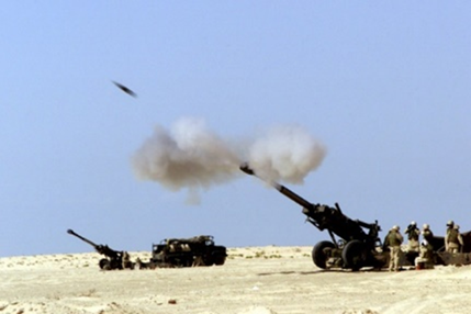
For instance, in ballistics, the dynamics of a particle \(P\) in the constant force field \(\overrightarrow{F}\) of the Earth is described by the equation \[\label{eq2.1} \frac{d\overrightarrow{p}}{dt} = \overrightarrow{F}, \tag{1}\] where \(\overrightarrow{p} = m \overrightarrow{v}\) is the momentum of the particle \(P\), \(m\) is the mass of \(P\), and \(\overrightarrow{v}\) is its velocity. The mass \(m\) of \(P\) is constant. In general, the velocity \(\overrightarrow{v}\) of \(P\) varies with time and is defined as \[\label{eq2.2} \overrightarrow{v} = \frac{d\overrightarrow{r}}{dt}. \tag{2}\]
In formula (2), \(\overrightarrow{r}(t)\) represents the position vector of the particle \(P\) at time \(t\) with respect to an arbitrarily chosen fixed reference frame.
In a particular reference system, appropriately chosen on the Earth’s surface, the differential equation (1) describing the motion of a shell fired from a cannon is written as \[\begin{aligned} \label{eq2.3}\begin{cases} \frac{d^{2}x}{dt^{2}} = 0,\quad x(0) = 0,\quad \frac{dx}{dt}(0) = 0,\\ \frac{d^{2}y}{dt^{2}} = 0,\quad y(0) = 0,\quad \frac{dy}{dt}(0) = v_{0} \cos\alpha,\\ \frac{d^{2}z}{dt^{2}} = -g,\quad z(0) = 0,\quad \frac{dz}{dt}(0) = v_{0} \sin\alpha.\end{cases} \end{aligned} \tag{3}\]
Its solution is \[\label{eq2.4} x(t) = 0,\quad y(t) = t v_{0} \cos\alpha,\quad z(t) = -\frac{g t^{2}}{2} + t v_{0} \sin\alpha. \tag{4}\]
Hence, the trajectory of the shell is given by \[\label{eq2.5} z = -\frac{g y^{2}}{2 v_{0}^{2} \cos^{2}\alpha} + y \tan\alpha. \tag{5}\]
For \(v_{0}=100~\mathrm{m/s}\) and \(\alpha=\pi/4\), the trajectory of the shell is presented in Figure 2.
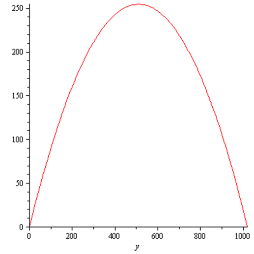
Figure 2 shows that the maximum distance reached by such a cannon and shell is approximately \(1020~\mathrm{m}\).
The presented description is objective, i.e., independent of the reference frame and the origin of time measurement. In general, the concept of an objective description in science means that the qualitative and quantitative descriptions of a given phenomenon remain unchanged when the phenomenon is observed by different observers; that is, it is possible to reconcile different observations of the process into a single coherent description.
Galileo Galilei (1564–1642) stated: “The mechanical event is independent of the observer. For frames moving uniformly with respect to each other, both states are mechanically equivalent.”
Isaac Newton (1643–1727) stated: “The mechanical event is independent of the observer. This also holds for accelerated systems if the frames of reference are fixed with respect to absolute space, that is, with respect to the fixed stars.”
Albert Einstein (1879–1955) stated: “The mechanical event is independent of the observer. There is no special reference point. The same holds for accelerated systems in general relativity.” Moreover, if a theory is subjected to relativity, it should be generally covariant under all transformations, not only under rigid-body motions. For further details concerning objectivity, see [8].
Moreover, the presented description is consistent.
Another example is the model that describes the motion of planets in the force field of the Sun. The description is made with respect to a particular reference frame whose origin is located at the center of the Sun, which is assumed to be a fixed point. The differential equation describing the motion of a planet of mass \(m\) is \[\label{eq2.6} \frac{d\overrightarrow{p}}{dt} = -\kappa \frac{m M}{|\overrightarrow{r}|^{3}} \overrightarrow{r}. \tag{6}\]
The computed trajectories are shown in Figure 3.
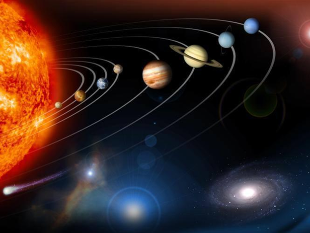
The presented description is objective, i.e., independent of the reference frame and the origin of time measurement. It allows astronomers to correlate observations made at different places and at different moments in time.
A constitutive law is a mathematical relationship that describes a material’s properties by connecting an applied force, such as stress, to the resulting deformation, such as strain. In physics and engineering, these laws define how a material behaves under certain conditions, such as elasticity, plasticity, or viscosity, based on its intermolecular forces and structure.
One example of a dynamical description that incorporates a constitutive law is the simple harmonic oscillator. This is an oscillator that is neither driven nor damped. It consists of a mass \(m\) that experiences a single force \(F\), which pulls the mass toward the point \(x = 0\) and depends only on the position \(x\) of the mass and the elastic constant \(k\). The balance of forces, according to Newton’s second law, for the system is given by \[\label{eq2.7} \frac{dp}{dt} = -k x. \tag{7}\]
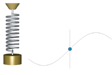
In practice, such a system is represented, for example, by the mass-spring harmonic oscillator shown in Figure 4.
Note that the constitutive law is incorporated into the right-hand side of Eq. (7). Eq. (7) is written with respect to a particular reference system whose axes are chosen in a specific way. The origin of the system is chosen to coincide with the point at which the tension in the spring, due to elongation, is equal to the force of gravity acting on the weight. More specifically, Eq. (7) is written as \[\begin{aligned} \label{eq2.8}\begin{cases} m \frac{d^{2}x}{dt^{2}} = -k x,\quad x(0) = x_{0},\quad \frac{dx}{dt}(0) = \dot{x}_{0},\\ m \frac{d^{2}y}{dt^{2}} = 0,\quad y(0) = 0,\quad \frac{dy}{dt}(0) = 0,\\ m \frac{d^{2}z}{dt^{2}} = 0,\quad z(0) = 0,\quad \frac{dz}{dt}(0) = 0.\end{cases} \end{aligned} \tag{8}\]
The solution of Eq. (8) is \[x(t) = A \sin\left(\sqrt{\frac{k}{m}}\, t + \varphi\right),\quad y(t) = 0,\quad z(t) = 0.\]
For \(k=1\), \(m=0.25\), \(x_{0}=0\), and 5\(\dot{x}_{0}=0.01\), the solution of Eq. (8) is \[x(t)=0.005\sin(2t),\quad y(t)=0,\quad z(t)=0.\] The function \(x(t)\) is shown in Figure 5.
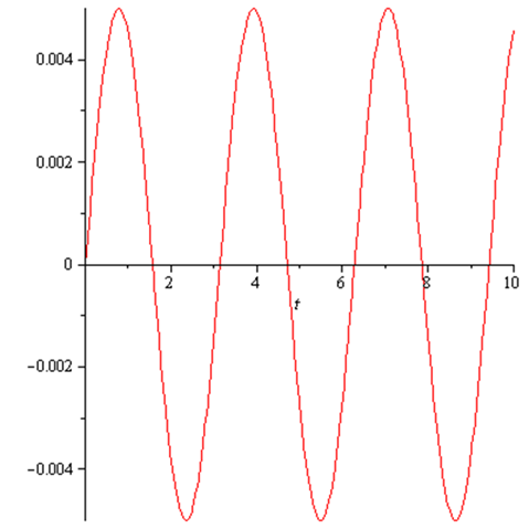
Note that this result was obtained using a particular reference frame and a particular origin for time measurement, but the result is independent of the choice of reference frame and the choice of the origin of time measurement. In terms of Galileo, Newton, and Einstein, this means that the description is objective. Moreover, the presented description is consistent. It should also be noted that the place where the constitutive law is incorporated, namely the right-hand side of the equation, does not affect the derivative of momentum.
In the following, objective and consistent descriptions of this type are presented in the field of fluid dynamics.
The Navier–Stokes momentum equation with constant viscosity for an incompressible fluid is \[\label{eq2.9} \rho \frac{\partial\overrightarrow{u}}{\partial t} + \rho (\overrightarrow{u} \cdot \nabla)\overrightarrow{u} = \nabla\left[-pI + \eta\left(\nabla\overrightarrow{u} + (\nabla\overrightarrow{u})^{T}\right)\right] + \overrightarrow{F}, \tag{9}\] together with \[\label{eq2.10} \nabla \cdot \overrightarrow{u} = 0, \tag{10}\] where \(\overrightarrow{u}\) is the fluid velocity, \(\rho\) is a constant representing the fluid density, \(p\) is the pressure, \(\eta\) is the viscosity, and \(\overrightarrow{F}\) represents the body forces.
Eq. (9) incorporates the constitutive law of constant viscosity, while Eq. (10) incorporates the constitutive law of incompressibility.
A first practical example of this type of description is the so-called “flow past a cylinder.” This example presents the time-dependent flow past a cylinder. The cylinder is placed slightly asymmetrically in the tube, and at a Reynolds number of about 100, a stream of vortices develops and forms a Karman vortex street. The equations describing the flow are Eqs. (9) and (10). The constitutive laws concerning the interaction between the fluid, the tube walls, and the cylinder wall are incorporated into the boundary conditions. The computed flow is presented in Figure 6.
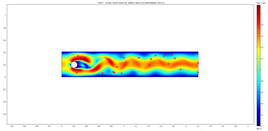
Note that this computed result was obtained using a particular reference frame and a particular origin for time measurement. However, it is independent of the reference frame and the origin of time measurement. This means that the description is objective in the Galileo–Newton–Einstein sense. Moreover, the presented description is consistent. It should also be noted that the constitutive laws are incorporated into the right-hand side of Eq. (9), which describes the dynamics, into the steady-state Eq. (10), which describes fluid incompressibility, and into the boundary conditions, such as the no-slip condition. Thus, this incorporation does not affect the derivative of momentum.
A more complex practical fluid-flow model is known as “ferrofluids as drug carriers in the human body.” Avoiding damage to healthy human cells caused by chemotherapy drugs imposes an upper limit on the treatment dose. This limit reduces the chances of successfully treating tumor cells. One objective of modern cancer research is therefore to concentrate chemotherapy drugs locally in tumor tissue and to reduce the global exposure of the organism. This model of the ferrohydrodynamics of blood demonstrates a simple setup for investigating an external magnetic field and its interaction with blood flow containing a magnetic carrier substance. The equations and theory are based on Maxwell’s equations and the Navier–Stokes equations.
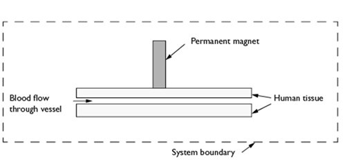
The model geometry represents a blood vessel, a permanent magnet, surrounding tissue, and air in two dimensions, as shown in Figure 7.
Blood enters the vessel from the left, as shown in Figure 7. The velocity and pressure fields are calculated in the bloodstream. The magnetic field generates a magnetic volume force that affects the flow field in the blood vessel.
Because the magnetic part of this problem is static, Maxwell–Ampere’s law for the magnetic field \(\mathbf{H}\) in \(\mathrm{A/m}\) and the current density \(\mathbf{J}\) in \(\mathrm{A/m^{2}}\) applies: \[\nabla \times \mathbf{H} = \mathbf{J}.\]
Furthermore, Gauss’ law for the magnetic flux density \(\mathbf{B}\) \((\mathrm{Vs/m^{2}})\) states that \[\nabla \cdot \mathbf{B} = 0.\] The constitutive equations describing the relation between \(\mathbf{B}\) and \(\mathbf{H}\) in the different parts of the modeling domain are given by \[\mathbf{B} = \begin{cases} \mu_0 \mu_{r,\mathrm{mag}} \mathbf{H} + \mathbf{B}_{\mathrm{rem}}, & \text{permanent magnet}, \\[4pt] \mu_0\left(\mathbf{H} + \mathbf{M}_{\mathrm{rf}}(\mathbf{H})\right), & \text{bloodstream}, \\[4pt] \mu_0 \mathbf{H}, & \text{tissue and air}. \end{cases}\]
Defining a magnetic vector potential \(\mathbf{A}\) such that \[\mathbf{B} = \nabla \times \mathbf{A}, \qquad \nabla \cdot \mathbf{A} = 0,\] one finally obtains the following vector equation to solve: \[\nabla \times \left( \frac{1}{\mu} \nabla \times \mathbf{A} – \mathbf{M} \right) = \mathbf{J}.\]
After simplifying the model to a two-dimensional problem with no perpendicular currents, this equation reduces to \[\nabla \times \left( \frac{1}{\mu_0} \nabla \times \mathbf{A} – \mathbf{M} \right) = 0.\] This equation assumes that the magnetic vector potential has a nonzero component only perpendicular to the plane, namely \[\mathbf{A} = (0,0,A_z).\]
A hyperbolic tangent expression with two material parameters, \(\alpha\) \((\mathrm{A/m})\) and \(\beta\) \((\mathrm{m/A})\), characterizes the induced magnetization \[\mathbf{M}_{\mathrm{ff},x,y} = (M_{\mathrm{ff},x},M_{\mathrm{ff},y})\] of a ferrofluid: \[M_x = \alpha \tanh \left( \frac{\beta}{\mu_0} \frac{\partial A_z}{\partial y} \right),\] \[M_y = \alpha \tanh \left( -\frac{\beta}{\mu_0} \frac{\partial A_z}{\partial x} \right).\]
For the magnetic fields of interest, it is possible to linearize these expressions to obtain \[M_x = \frac{\chi}{\mu_0} \frac{\partial A_z}{\partial y},\] \[M_y = -\frac{\chi}{\mu_0} \frac{\partial A_z}{\partial x}.\]
Along a system boundary located sufficiently far from the magnet, one can apply the magnetic insulation boundary condition \[A_z = 0.\]
The Navier–Stokes equations describe the time-dependent mass and momentum balances for incompressible flow: \[\rho \frac{\partial \mathbf{u}}{\partial t} – \nabla \cdot \eta \left( \nabla \mathbf{u} + (\nabla \mathbf{u})^{T} \right) + \rho \mathbf{u} \cdot \nabla \mathbf{u} + \nabla p = \mathbf{F},\] \[\nabla \cdot \mathbf{u} = 0,\] where \(\eta\) denotes the dynamic viscosity \((\mathrm{kg/(m\cdot s)})\), \(\mathbf{u}\) is the velocity \((\mathrm{m/s})\), \(\rho\) is the fluid density \((\mathrm{kg/m^{3}})\), \(p\) is the pressure \((\mathrm{N/m^{2}})\), and \(\mathbf{F}\) is a volume force \((\mathrm{N/m^{3}})\).
Under the assumption that the magnetic nanoparticles in the fluid do not interact, the magnetic force \(\mathbf{F}=(F_x,F_y)\) acting on the ferrofluid in relatively weak fields is given by \[\mathbf{F} = |\mathbf{M}\nabla \mathbf{H}|.\] Hence, \[F_x = \frac{\chi}{\mu_0 \mu_r^2} \left( \frac{\partial A_z}{\partial x} \frac{\partial^2 A_z}{\partial x^2} + \frac{\partial A_z}{\partial y} \frac{\partial^2 A_z}{\partial x \partial y} \right),\] \[F_y = \frac{\chi}{\mu_0 \mu_r^2} \left( \frac{\partial A_z}{\partial x} \frac{\partial^2 A_z}{\partial x \partial y} + \frac{\partial A_z}{\partial y} \frac{\partial^2 A_z}{\partial y^2} \right).\]
To obtain the final expression for the volume force in the bloodstream, these expressions are multiplied by the ferrofluid mass fraction, \(k_{\mathrm{ff}}\).
On the vessel walls, no-slip conditions are applied: \[u = v = 0.\] At the outlet, an outlet pressure condition can be prescribed: \[p = 0.\] At the inlet boundary, a parabolic flow profile is specified for the normal inflow velocity according to \(4U_m s(1-s)\), where \(s\) is a boundary-segment length parameter varying from \(0\) to \(1\) along the inlet boundary segment, and \(U_m\) is the maximum flow velocity. To emulate the heartbeat, the inflow velocity follows a sinusoidal expression in time: \[U_0 = 2U_m s(1-s) \left( \sin \omega t + \sqrt{\sin^2(\omega t)} \right).\]
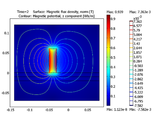
Selecting the angular velocity \(\omega\) as \(2\pi~\mathrm{rad/s}\) gives a heartbeat rate of \(60\) beats per minute. Some of the computed quantities are shown in Figures 8–10.
Note that this result was obtained using a particular reference frame and a particular origin for time measurement. However, the result is independent of the reference frame and the origin of time measurement. This means that the description is objective. Moreover, the presented description is consistent. The place where the constitutive laws are incorporated does not affect the derivative of impulse.
We continue with the presentation of objective and consistent descriptions in the field of heat transport processes.
There are three main heat-transfer processes:
The governing transient and steady-state equations for this process are \[\label{eq11} \rho C_{\rho} \frac{\partial T}{\partial t} + \nabla(-k\nabla T) = Q, \tag{11}\] and \[\label{eq12} \nabla(-k\nabla T) = Q. \tag{12}\]
The governing transient and steady-state equations for this process are \[\label{eq13} \rho C_{\rho} \frac{\partial T}{\partial t} + \nabla(-k\nabla T) = Q – \rho C_{\rho} \mathbf{u} \cdot \nabla T, \tag{13}\] and \[\label{eq14} \nabla(-k\nabla T) = Q – \rho C_{\rho} \mathbf{u} \cdot \nabla T. \tag{14}\]
The governing transient and steady-state equations for this process are \[\label{eq15} \rho C_{\rho} \frac{\partial T}{\partial t} + \nabla(-k\nabla T) = Q – \rho C_{\rho} \mathbf{u} \cdot \nabla T – \frac{\varepsilon \sigma p}{A} T^{4}, \tag{15}\] and \[\label{eq16} \nabla(-k\nabla T) = Q – \rho C_{\rho} \mathbf{u} \cdot \nabla T – \frac{\varepsilon \sigma p}{A} T^{4}. \tag{16}\]
Eqs. (11)–(16) are independent of the reference frame and the origin of time measurement. This means that the description is objective in the Galileo–Newton–Einstein sense. Moreover, the presented descriptions are consistent. It should also be noted that the places where the constitutive laws are incorporated, namely the right-hand sides and boundary conditions, do not affect the derivative of impulse.
Some applications of the above heat-transport equations to real-world phenomena are presented below:
This model describes the nonisothermal flow of argon gas inside a light bulb. The purpose of the model is to show the coupling between energy transport, through conduction and convection, and momentum transport induced by density variations in the argon gas. The model geometry is shown in Figure 11.
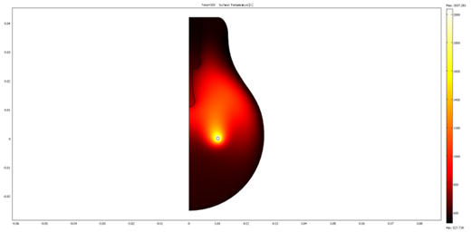
The governing equations of the process are \[\rho C_{\rho} \frac{\partial T}{\partial t} + \nabla(-k\nabla T) = Q + q_{s} T,\] \[\rho \frac{\partial\overrightarrow{u}}{\partial t} +\rho \left( \overrightarrow{u}\cdot\nabla \right)\overrightarrow{u} = \nabla\left[ -pI +\eta\left( \nabla\overrightarrow{u} +\left( \nabla\overrightarrow{u} \right)^{T} \right) -\left( \frac{2\eta}{3} – k_{dv} \right) \left( \nabla\cdot\overrightarrow{u} \right)I \right] +\overrightarrow{F},\] \[\frac{\partial\rho}{\partial t} + \nabla\cdot(\rho \overrightarrow{u}) = 0,\] and \[\rho = \rho(p,T).\]
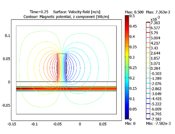
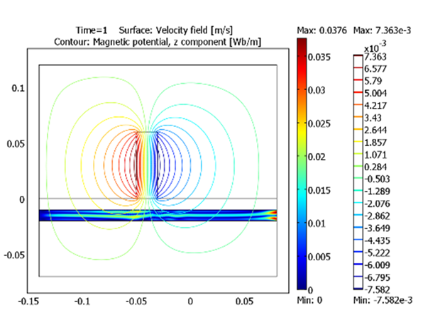
This is a stationary model of a heating circuit, including DC-induced Joule heating, heat transfer, and structural-mechanics analysis of the thin resistive layer covering a solid glass plate. The model is shown in Figure 12.
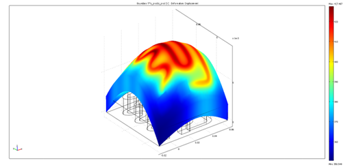
The governing equation of the process is \[\nabla(-k \nabla T) = Q + q_{s} T.\]
A thin microwave antenna is inserted into a tumor. The microwaves heat the tumor, producing a coagulated region in which cancer cells are killed. The model is shown in Figure 13.
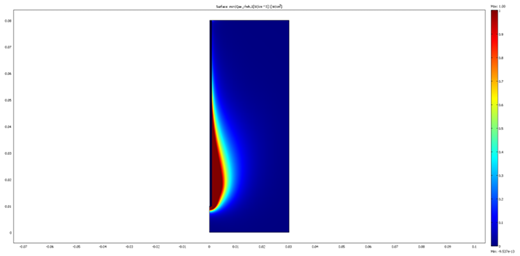
The governing equation of the process is \[\nabla(-k\nabla T) = \rho_{b} C_{b} \omega_{b}(T_{b}-T) + Q_{\mathrm{met}} + Q_{\mathrm{ext}}.\]
The bioheat equation is \[\nabla \times \left[ \left( \varepsilon_{r} – j\frac{\sigma}{\omega \varepsilon_{0}} \right)^{-1} \nabla \times \overrightarrow{H} \right] – \mu_{r} k_{0}^{2}\overrightarrow{H} =0, \qquad \overrightarrow{H}=H_{\varphi}\overrightarrow{e}_{\varphi}, \qquad \varepsilon_{r}=n^{2},\] for TM waves.
This model describes an aluminum heat sink mounted on a processor with a given power. To prevent overheating, cool air is pumped through the microchannels of the heat sink. The model is shown in Figure 14.
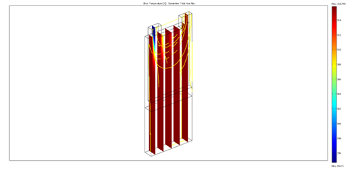
The governing equations of the process are \[\nabla(-k\nabla T)=Q+q_{s}T,\] \[\rho \left( \overrightarrow{u}\cdot\nabla \right)\overrightarrow{u} = \nabla\left[ -pI +\eta\left( \nabla\overrightarrow{u} + \left(\nabla\overrightarrow{u}\right)^{T} \right) – \left( \frac{2\eta}{3}-k_{dv} \right) \left(\nabla\cdot\overrightarrow{u}\right)I \right] + \overrightarrow{F},\] \[\nabla\cdot(\rho\overrightarrow{u})=0.\]
The model describes the temperature field and fluid flow in a cylindrical power transformer, including variations in fluid properties with temperature. The model is shown in Figure 15.
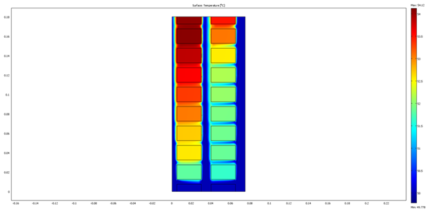
The governing equations of the process are \[\nabla(-k\nabla T)=Q+q_{s}T,\] \[\rho \left( \overrightarrow{u}\cdot\nabla \right)\overrightarrow{u} = \nabla\left[ -pI +\eta\left( \nabla\overrightarrow{u} + \left(\nabla\overrightarrow{u}\right)^{T} \right) – \left( \frac{2\eta}{3}-k_{dv} \right) \left(\nabla\cdot\overrightarrow{u}\right)I \right] + \overrightarrow{F},\] \[\nabla\cdot(\rho\overrightarrow{u})=0.\]
The inductor is a common component in a variety of electrical devices. Its applications include power transformation and measurement, and it can also be used together with capacitors to create oscillators. In small devices with many components, such as laptops, heat generation can be a problem and must be accounted for in the design. This axisymmetric two-dimensional model studies heat transfer in a potcore inductor. It solves for heat transfer inside the inductor and in the surrounding air, as well as for the airflow around the inductor. The model is shown in Figure 16.
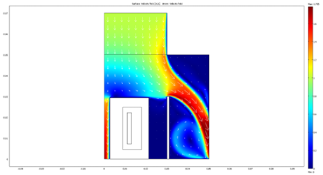
The governing equations of the process are \[\nabla(-k\nabla T)=Q+q_{s}T,\] \[\rho \left( \overrightarrow{u}\cdot\nabla \right)\overrightarrow{u} = \nabla\left[ -pI +\eta\left( \nabla\overrightarrow{u} + \left(\nabla\overrightarrow{u}\right)^{T} \right) – \left( \frac{2\eta}{3}-k_{dv} \right) \left(\nabla\cdot\overrightarrow{u}\right)I \right] + \overrightarrow{F},\] \[\nabla\cdot(\rho\overrightarrow{u})=0.\]
This model consists of the merger of two components: a heating device and an aluminum heat sink. The assembly of these components simulates the measuring setup for heat sinks from Alpha Company Ltd. in Japan. The model is shown in Figure 17.
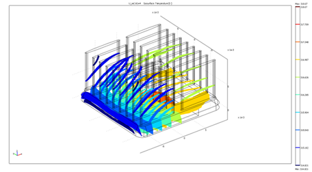
The governing equation of the process is \[\nabla(-k\nabla T)=Q.\]
The following examples concern models for electric-charge transport and electromagnetic-wave propagation.
A cold crucible is modeled for the manufacturing of alloys that require a high degree of purity. The cold crucible is surrounded by an inductor, which makes the crucible act as a “field concentrator” because of the induced currents. The model is shown in Figure 18.
The governing equation of the process is \[\left( j\omega\sigma – \omega^{2}\varepsilon_{0}\varepsilon_{r} \right)\overrightarrow{A} + \nabla \times \left( \mu_{0}^{-1}\mu_{r}^{-1} \nabla \times \overrightarrow{A} \right) = \overrightarrow{J}^{e}.\]
The boundary conditions are \[\overrightarrow{n}\times\overrightarrow{A}=0,\] which represents magnetic insulation; \[\overrightarrow{n}\times\overrightarrow{H}=0,\] which represents electric insulation; \[-\overrightarrow{n}\times\overrightarrow{H} = \overrightarrow{J}_{s},\] which represents a surface current; and \[\left( \frac{\mu_{0}\mu_{r}} {\varepsilon_{0}\varepsilon_{r}-\frac{j\sigma}{\omega}} \right)^{1/2} \overrightarrow{n}\times\overrightarrow{H} + \overrightarrow{E} – (\overrightarrow{n}\cdot\overrightarrow{E})\overrightarrow{n} = (\overrightarrow{n}\cdot\overrightarrow{E}_{s})\overrightarrow{n} – \overrightarrow{E}_{s},\] which represents the impedance boundary condition.
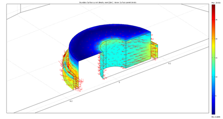
The eddy currents in a conductive cylinder, generated by currents passing through a surrounding coil, are modeled. The skin effect in the coil is also studied. The model is shown in Figure 19.
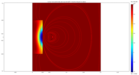
The governing equations of the process are \[\left( j\omega\sigma – \omega^{2}\varepsilon_{0}\varepsilon_{r} \right)\overrightarrow{A} + \nabla \times \left( \mu_{0}^{-1}\mu_{r}^{-1}\nabla \times \overrightarrow{A} \right) – \sigma\overrightarrow{v} \times \left( \nabla \times \overrightarrow{A} \right) = \left( \frac{\sigma V_{\mathrm{loop}}}{2n_{r}} + J_{\varphi}^{e} \right)\overrightarrow{e}_{\varphi},\] \[\overrightarrow{A}=A_{\varphi}\overrightarrow{e}_{\varphi}.\]
The boundary conditions are \[\overrightarrow{n}\cdot \left( \overrightarrow{H}_{1}-\overrightarrow{H}_{2} \right) = J_{\mathrm{sp}},\] which represents the surface current density; \[A_{\varphi}=0,\] which represents magnetic insulation; \[\overrightarrow{n}\cdot \left( \overrightarrow{H}_{1}-\overrightarrow{H}_{2} \right) = 0,\] which represents continuity; and \[r=0,\] which represents axial symmetry.
This is an example of how to model perfectly matched layers. The model shows scattering from a dielectric object and how the scattered wave is absorbed by PMLs. The model is shown in Figure 20.
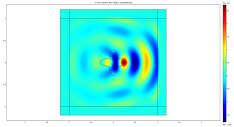
The governing equation of the process is \[\nabla \times \left( \mu_{r}^{-1}\nabla \times \overrightarrow{E} \right) – \left( \varepsilon_{r} – \frac{j\sigma}{\omega\varepsilon_{0}} \right) k_{0}^{2}\overrightarrow{E} = 0, \qquad \overrightarrow{E}=E\overrightarrow{e}_{z}, \qquad \varepsilon_{r}=n^{2}.\]
The scattering boundary condition for a plane wave is \[\overrightarrow{n}\times \left( \nabla \times \overrightarrow{E} \right) – jk_{\mathrm{sc}}\overrightarrow{E} = 0.\]
This model shows how to calculate the far-field radiation pattern from an antenna. The model is shown in Figure 21.
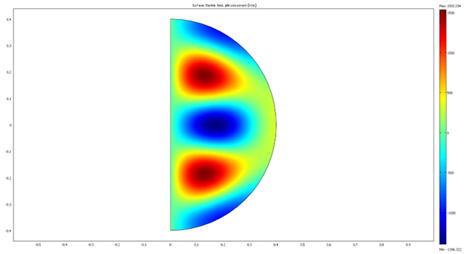
The governing equation of the process is \[\nabla \times \left( \mu_{r}^{-1}\nabla \times \overrightarrow{E} \right) – \left( \varepsilon_{r} – \frac{j\sigma}{\omega\varepsilon_{0}} \right) k_{0}^{2}\overrightarrow{E} = 0, \qquad \overrightarrow{E}=E_{\varphi}\overrightarrow{e}_{\varphi}, \qquad \varepsilon_{r}=n^{2}.\]
The boundary conditions are \[r=0,\] which represents axial symmetry, and \[\overrightarrow{n}\cdot \left( \nabla \times E_{\varphi} \right) – jkE_{\varphi} = 0,\] which represents the scattering boundary condition for a spherical wave.
The Schumann resonance frequencies are a set of eigenmodes in the extremely low-frequency (ELF) portion of the electromagnetic-field spectrum. These resonance frequencies are present only for planet-like bodies with a substantial ionosphere. The ionosphere acts as a perfect electric conductor enclosing a resonance cavity together with the surface. This model computes the Schumann resonance frequencies for the Earth. The model is shown in Figure 22.
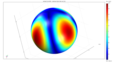
The governing equation of the process is \[\nabla \times \left( \mu_{r}^{-1}\nabla \times \overrightarrow{E} \right) – \left( \varepsilon_{r} – \frac{j\sigma}{\omega\varepsilon_{0}} \right) k_{0}^{2}\overrightarrow{E} = 0, \qquad \varepsilon_{r}=n^{2}, \qquad \lambda=-j\omega+\delta.\]
The boundary condition is \[\overrightarrow{n}\cdot\overrightarrow{E}=0,\] which represents a perfect electric conductor.
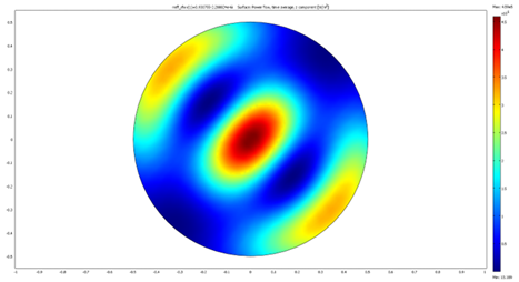
This model shows how to set up a mode analysis with lossy metallic walls for a waveguide. The attenuation, measured in \(\mathrm{dB/km}\), is extracted for several modes. The model is shown in Figure 23.
The governing equation of the process is \[\begin{aligned} &\nabla \times \left( n^{2}\nabla \times \overrightarrow{H} \right) – k_{0}^{2}\overrightarrow{H} = 0, \\ &\overrightarrow{H} = \overrightarrow{H}(x,y)\exp(\lambda z), \quad \varepsilon_{r}=n^{2}, \quad \mu_{r}=1, \quad \sigma=0, \quad \lambda=-j\beta-\delta_{z}. \end{aligned}\]
The boundary condition is
\[- \left( \varepsilon-\frac{j\sigma}{\omega} \right)^{1/2} \overrightarrow{n}\times\overrightarrow{E} + \mu^{1/2} \overrightarrow{n}\times \left( \overrightarrow{H}\times\overrightarrow{n} \right) = 0.\] This represents the impedance boundary condition for a plane wave.
In the above examples, the equations were solved in particular reference frames. However, the obtained results are independent of the reference frame and the origin of time measurement. This means that the descriptions are objective in the Galileo–Newton–Einstein sense. Moreover, the presented descriptions are consistent. It should also be noted that the places where the constitutive laws are incorporated, namely the right-hand sides and boundary conditions, do not affect the derivative of impulse.
Lastly, there are what may be termed “hypothetical” laws, which are based on qualitative reasoning in the absence of precise rules. For example, in the Lotka–Volterra model of interacting predator and prey populations, the death rate of the prey is assumed to be proportional to the product of the two populations. This is a phenomenological assumption that is plausible and is similar to the law of mass action in chemical reactions, although it has no direct quantitative basis. In this case, the usefulness of the model lies in explaining the mechanism by which interacting populations can oscillate. These types of descriptions are also objective.
The competitive Lotka–Volterra equations are a simple model of the population dynamics of species competing for a common resource. They can be further generalized to include trophic interactions.
The form is similar to the Lotka–Volterra equations for predation, in that the equation for each species contains one term for self-interaction and one term for interaction with other species. In the equations for predation, the basic population model is exponential. For the competition equations, the logistic equation is the basis. The logistic population model, when used by ecologists, often takes the following form: \[\label{eq17} \frac{dx}{dt} = r x \left(1 – \frac{x}{K}\right). \tag{17}\]
Here, \(x\) is the size of the population at a given time, \(r\) is the intrinsic per-capita growth rate, and \(K\) is the carrying capacity.
Given two populations, \(x_{1}\) and \(x_{2}\), with logistic dynamics, the Lotka–Volterra formulation adds an additional term to account for the interactions between species. Thus, the competitive Lotka–Volterra equations are \[\label{eq18} \frac{dx_{1}}{dt} = r_{1}x_{1} \left( 1-\frac{x_{1}+\alpha_{12}x_{2}}{K_{1}} \right), \tag{18}\] and \[\label{eq19} \frac{dx_{2}}{dt} = r_{2}x_{2} \left( 1-\frac{x_{2}+\alpha_{21}x_{1}}{K_{2}} \right). \tag{19}\]
Here, \(\alpha_{12}\) represents the effect that species 2 has on the population of species 1, and \(\alpha_{21}\) represents the effect that species 1 has on the population of species 2. These values do not have to be equal. Because this is the competitive version of the model, all interactions are harmful, and therefore all \(\alpha\)-values are positive. It should also be noted that each species can have its own growth rate and carrying capacity.
This model can be generalized to any number of species competing with one another.
Eqs (18) and (19) are independent of the reference frame and the origin of time measurement.
For \[r_{1}=1,\quad r_{2}=0.75,\quad \alpha_{12}=1.09,\quad \alpha_{21}=0.50, \quad K_{1}=1,\quad K_{2}=1,\] some computed results are presented in Figure 24.
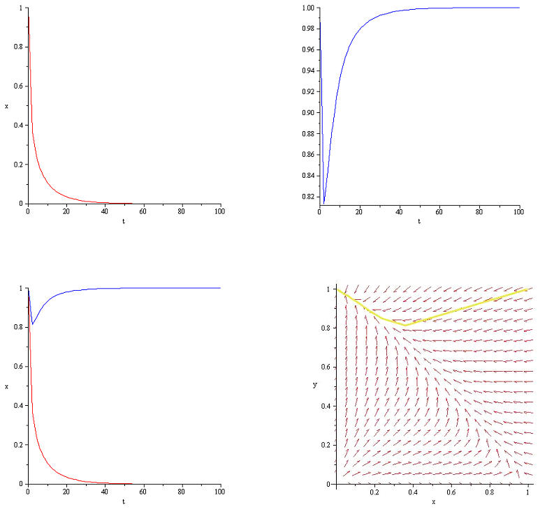
The obtained results are independent of the reference frame and the origin of time measurement. This means that the description is objective in the Galileo–Newton–Einstein sense. Moreover, the presented description is consistent. It should also be noted that the place where the “hypothetical” laws are incorporated, namely the right-hand side of the equations, does not affect the time-dependent derivative of the population sizes.
A power law is a functional relationship between two quantities in which a relative change in one quantity results in a relative change in the other quantity proportional to the first change raised to a constant exponent. In other words, one quantity varies as a power of another. This change is independent of the initial size of the quantities. For instance, the area of a square has a power-law relationship with the length of its side, since if the length is doubled, the area is multiplied by \(2^{2}\), while if the length is tripled, the area is multiplied by \(3^{2}\), and so on [9].
The distributions of a wide variety of physical, biological, and human-made phenomena approximately follow a power law over a wide range of magnitudes. These include the sizes of craters on the Moon and solar flares [10], cloud sizes [11], the foraging patterns of various species [12], the sizes of activity patterns of neuronal populations [13], the frequencies of words in most languages, the frequencies of family names, species richness in clades of organisms [14], the sizes of power outages and volcanic eruptions [15], human judgments of stimulus intensity [16, 17], and many other quantities [18]. Empirical distributions can fit a power law only over a limited range of values, because a pure power law would allow arbitrarily large or small values. Acoustic attenuation follows frequency power laws within wide frequency bands for many complex media. Allometric scaling laws for relationships between biological variables are among the best-known power-law functions in nature.
More than a hundred power laws have been identified in physics, biology, and the social sciences. Among them are the following: in artificial intelligence, neural scaling laws; in astronomy, Kepler’s third law, the initial mass function of stars, the differential energy spectrum of cosmic-ray nuclei, the M–sigma relation, and solar flares; in biology, Kleiber’s law relating animal metabolism to size, allometric laws in general, the two-thirds power law relating speed to curvature in the human motor system, Taylor’s law relating mean population size and variance of population size in ecology, neuronal avalanches, species richness in clades of freshwater fishes, the Harlow–Knapp effect, the size distribution of forest patches globally, and the species–area relationship relating the number of species found in an area to the size of that area; in chemistry, rate laws; in climate science, the sizes of cloud areas and perimeters as viewed from space, the sizes of rain-shower cells, energy dissipation in cyclones, and the diameters of dust devils on Earth and Mars; in general science, highly optimized tolerance, proposed forms of experience-curve effects, pink noise, the law of stream numbers and the law of stream lengths in Horton’s laws describing river systems, populations of cities according to Gibrat’s law, bibliograms and word-frequency distributions in texts according to Zipf’s law, the 90–9–1 principle on wikis, also referred to as the 1% rule, Richardson’s law for the severity of violent conflicts such as wars and terrorism, the relationship between CPU cache size and the number of cache misses, the spectral density of the weight matrices of deep neural networks, tails in statistical distributions for exponential growth processes with random observation or killing, and progress through exponential growth and exponential diffusion of innovations.
In economics, examples include population sizes of cities in a region or urban network, Zipf’s law, the distribution of artists by the average price of their artworks, income distribution in a market economy, the distribution of degrees in banking networks, firm-size distributions, and scaling laws of socioeconomic quantities with respect to population size, such as urban scaling. In finance, examples include returns for high-risk venture-capital investments, the mean absolute change of logarithmic mid-prices, large price changes, volatility and transaction volume on stock exchanges, the average waiting time of a directional change, and the average waiting time of an overshoot.
In mathematics, examples include fractals, the Pareto distribution and the Pareto principle, also called the “80–20 rule,” Zipf’s law in corpus analysis and population distributions, the zeta distribution, the Yule–Simon distribution, Student’s \(t\)-distribution, of which the Cauchy distribution is a special case, Lotka’s law, and the scale-free network model. In physics, examples include the Ångström exponent in aerosol optics, the frequency dependence of acoustic attenuation in complex media, the Stefan–Boltzmann law, the input-voltage–output-current curves of field-effect transistors and vacuum tubes, which approximate a square-law relationship, the square–cube law relating surface area to volume, the \(3/2\)-power law in the plate characteristic curves of triodes, the inverse-square laws of Newtonian gravity and electrostatics, self-organized criticality with a critical point as an attractor, models of van der Waals forces, force and potential in simple harmonic motion, gamma correction relating light intensity to voltage, behavior near second-order phase transitions involving critical exponents, the safe operating area relating maximum simultaneous current and voltage in power semiconductors, supercritical states of matter and supercritical fluids, the Curie–von Schweidler law in dielectric responses to step DC voltage input, the damping-force–speed relation in antiseismic damper calculations, and folded solvent-exposed surface areas of centered amino acids in protein-structure segments.
In political science, an example is the cube-root law of assembly sizes. In psychology, examples include Stevens’s power law of psychophysics and the power law of forgetting.
The ratio of the square of a planet orbital period with the cube of the semi-major axis of its orbit is the same for all planets orbiting the Sun.
\[\label{eq20} \frac{a^{3}}{T^{2}} = 7.496 \quad \text{or} \quad T = \frac{1}{\sqrt{7.496}} a^{3/2}. \tag{20}\]
Upon finding this pattern Kepler wrote [19]: ’I first believed I was dreaming… But it is absolutely certain and exact that the ratio which exists between the period times of any two planets is precisely the ratio of the 3/2th power of the mean distance’, translated from Harmonies of the World by Kepler (1619). The data used by Kepler (1618) is given in Table 1 and the modern data is given in Table 2.
| Planet | Mean distance to sun (AU) | Period(days) | R3T2 (10-6 AU3/day2) |
|---|---|---|---|
| Mercury | 0.389 | 87.77 | 7.64 |
| Venus | 0.724 | 224.7 | 7.52 |
| Earth | 1 | 365.25 | 7.5 |
| Mars | 1.524 | 686.95 | 7.5 |
| Jupiter | 5.2 | 4332.6 | 7.49 |
| Saturn | 9.51 | 10759 | 7.43 |
| Planet | Semi-major axis (AU) | Period (days) | a3T2 (10-6 AU3/day2) |
|---|---|---|---|
| Mercury | 0.38710 | 87.9693 | 7.496 |
| Venus | 0.72333 | 224.7008 | 7.496 |
| Earth | 1 | 365.2564 | 7.496 |
| Mars | 1.52366 | 686.9796 | 7.495 |
| Jupiter | 5.20336 | 4332.8201 | 7.504 |
| Saturn | 9.53707 | 10775.599 | 7.498 |
| Uranus | 19.1913 | 30687.153 | 7.506 |
| Neptune | 30.0690 | 60190.03 | 7.504 |
Isaac Newton computed in his PhilosophiæNaturalis Principia Mathematica the acceleration of a planet moving according to Kepler’s first and second laws.
The direction of the acceleration is towards the Sun.
The magnitude of the acceleration is inversely proportional to the square of the planet’s distance from the Sun (the inverse square law).
This implies that the Sun may be the physical cause of the acceleration of planets. However, Newton states in his Principia that he considers forces from a mathematical point of view, not a physical, thereby taking an instrumentalist view [20]. Moreover, he does not assign a cause to gravity [21].
Newton defined the force acting on a planet to be the product of its mass and the acceleration (see Newton’s laws of motion). So:
Every planet is attracted towards the Sun.
The force acting on a planet is directly proportional to the mass of the planet and is inversely proportional to the square of its distance from the Sun.
The Sun plays an unsymmetrical part, which is unjustified. So he assumed, in Newton’s law of universal gravitation:
All bodies in the Solar System attract one another.
The force between two bodies is in direct proportion to the product of their masses and in inverse proportion to the square of the distance between them.
As the planets have small masses compared to that of the Sun, the orbits conform approximately to Kepler’s laws. Newton’s model improves upon Kepler’s model, and fits actual observations more accurately.
Remark that Kepler’s power law in astronomy first was found by Kepler using experimental data and later it was deduced in the framework of a mental construction which is called today Newton’s Mechanics. For details deriving Kepler’s power law using first and second order derivatives see [22], pg.175.
Curie-von Schweidler law refers to the response of dielectric material to the step input of a direct current (DC) voltage first observed by Jacques Curie [23, 24] and Egon Ritter von Schweidler [25]. The Curie current represents the response of a dielectric material to a step input DC voltage. According to [23],[24] the J. Curie current intensity is given by \[i_{Curie}(t) = V_{0} \frac{t^{-\alpha}}{h}, \tag{21}\] where \(0 < \alpha < 1\) is a constant, \(V_{0}\) is a constant representing the magnitude of the step input DC voltage; \(h\) is a constant related to the capacitance of the capacitor and the kind of dielectric.
In [25] von Schweidler presents the main forms of abnormal behavior of dielectrics as follows.
If the terminals of a capacitor are connected to the poles of a current source with constant electromotive force, a current will appear in the conductors, the intensity of which decreases with time. For an ideal non-conducting dielectric, according to the general theory, the following differential equation applies to the “normal charging current”:
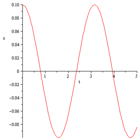
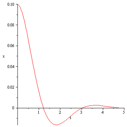
\[L \frac{d^{2}i}{dt^{2}} + R \frac{di}{dt} + \frac{1}{C} i = 0, \tag{22}\] where \(C\) is the capacitance of the capacitor, \(L\) the self-inductance coefficient, and \(R\) the resistance of the external circuit. Depending on the ratio of the numerical values of these three constants, the charging of the capacitor occurs either oscillatory or aperiodically. With a relatively small resistance of the external circuit, the current in each of the two traps decreases very rapidly, so that in practically realizable traps the normal charging current can be set to zero after times of the order of a small fraction of a second.
If the dielectric is not perfectly insulating, then a normal conduction current ’a’ is superimposed on the normal charging current, ’a’ is given by the formula
\[a = \frac{4\pi\lambda}{K} C E, \tag{23}\] where \(\lambda\) is the specific conductance, \(K\) is the dielectric constant of the medium, \(C\) is the capacitance of the capacitor and \(E\) is the electromotive force of the current source (all quantities are considered to be measured in absolute electrostatic units).
In fact, as can be seen, in many dielectrics, besides the normal charging current and the normal conduction current, there is another “anomalous charging current” that overlaps, so that the entire current can be represented by:
\[J_{1} = i_{1} + y_{1} + a.\]
Here, \(y_{1}\) is a function of time that asymptotically decreases to zero, but it is much more complex than the normal load current \(i_{1}\).
Oscillatory charging for \(R=0\), \(L=1\), and \(C=0.25\) is shown in Figure 25, while aperiodic charging for \(R=2\), \(L=1\), and \(C=0.25\) is shown in Figure 26.
If the terminals of the capacitor are connected together after being maintained at a constant potential difference for a time interval \(\delta\), then two Open must be distinguished in terms of the laws of the discharge current:
a) The discharge current \(J_{2}\) corresponds to the normal discharge current \(i_{2}\), which is determined by an analogous integer differential equation, like the normal load current \(i_{1}\);
b) Analogous to the load, an “anomalous discharge current” \(y_{2}\) is superimposed, and \(y_{2}\) is again a function of it that decreases to zero with increasing time. The following relationship between \(y_{1}\) and \(y_{2}\) is also valid:
\[\int_{0}^{\delta} y_{1} dt = -\int_{0}^{\infty} y_{2} dt. \tag{25}\]
That is, the total amount of electricity passing through a cross section of the conductor as a result of the abnormal discharge current is equal to the amount that was carried by the abnormal charge current during the charging period \(\delta\).
In case a), which is carried out especially with various poorly conductive liquids (Koller; Schweidler; Gadeke), the charging process proceeds as if the conductivity of the medium were undergoing temporal changes due to the passage of current. In case b), the charging process is reversible; the medium behaves as if the conductivity corresponding to the time integral of the abnormal charging current \(\int_{0}^{\delta} y_{1} dt\). The amount of electricity absorbed is gradually released again during the discharge. This reversible process is usually referred to as the formation or pre-production of the “residue”, and the integral \(\int_{0}^{\delta} y_{1} dt\) dt as the “residual charge” formed during time \(\delta\).
In principle, the situation is less simple when the capacitor terminals are not held at constant potentials, but one of them is isolated; however, this form of residual phenomenon is historically the main one and this has led to the aforementioned name. If a capacitor is charged and then one of the two terminals is isolated, the potential difference V between the terminals, and therefore the so-called “dissipative charge” given by the product CV, decreases. This decrease occurs more rapidly than would correspond to the constant conduction current ’a’. Conversely, if the charged capacitor is discharged by temporarily connecting the terminals and only one terminal is isolated, a new charge of the same sign as the original gradually appears, increases to a maximum and then (due to the conduction of the dielectric) decreases asymptotically to zero.
Regarding the laws that apply to the temporal evolution of residual phenomena and their dependence on other constraints, experimental investigations have led to the following results:
The anomalous charging current or residue formation current \(y_{1}\), at the terminals of a given capacitor with a given electromotive force, can be represented as a function of time by:
\[y_{1} = B t^{-n},\quad n < 1. \tag{26}\]
This formula can only be considered an approximation, because initially, we obtain for \(t = 0\), \(y_{1} = \infty\). But formula \[\int_{0}^{\delta} y_{1} dt=\frac{B \times t^{1-n}}{1-n},\] make sense because for finite \(\delta\) the integral remains finite. Moreover for \(t=\infty\), \[\int_{0}^{\delta} y_{1} dt=\infty.\] Which is also unlikely. The current in the first infinitely small time element, as well as after an infinitely long time, cannot, of course, be determined empirically. In the time intervals accessible to observation, the above formula has been well confirmed (Kohlrausch; Hopkinson; Giese; J. Curie, I, 21 et al.).
If the same capacitor is examined under the influence of different electromotive forces, the following results:
\[y_{1} = B t^{-n} = b E t^{-n}. \tag{27}\]
The residual current \(y_1\) of the electromotive force E is proportional to the current, assuming that the evolution over time remains unchanged. (Kohlrausch; J. Curie).
If a given dielectric is examined in layers of different thicknesses, then according to Hopkinson, the residual current \(y_{1}\) is inversely proportional to the thickness, again with an unchanged time evolution. Since the proportionality of the current to the cross-sectional area (coverage area) is obvious, one can set the current proportional to the capacitance of the ionic capacitor and obtain the formula:
\[y_{1} = b E t^{-n} = \beta C E t^{-n}, \tag{28}\] where now \(\beta\) and \(n\) are constants of the environment as such.
The following law applies to the discharge current:
After a very long charging time of the capacitor, the discharge current \(y_{2}\) is equal to and opposite to the charging current.
\[y_{2} = -y_{1}. \tag{29}\]
For a shorter loading time, \(\delta\), \(y_{2} < y_{1}\), shows a faster decrease in time, which can be represented by the formula:
\[y_{1} = f(t) = B t^{-n}, \tag{30}\] \[y_{2} = -f(t) + f(t + \delta), \tag{31}\] where \(t\) is the time measured from the beginning of charging (at \(y_{1}\)) or discharging (at \(y_{2}\)), and \(\delta\) is the duration of charging.
This result can be interpreted as follows: The observed discharge current \(y_{2}\) comes from the superposition of the current \(-f(t)\), which opposes the charging current \(y_{1} = f(t)\), and a current \(f(t + \delta)\), which can be considered simply the undisturbed continuation of the charging current even after discharge. This so-called principle of superposition was discovered experimentally by Hopkinson and J. Curie.
The formula mentioned above, \(-\int_0^{\delta}y_1dt=\int_0^{\infty}y_2dt\), is a consequence of the same principle.
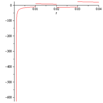
Therefore, if at times \(t = \delta_{1}, \delta_{2}, \delta_{3}, \ldots, \delta_{k}\), jumps of the potential difference with the values (positive or negative): \(E_{1}, E_{2}, E_{3}, \ldots, E_{k}\) occur then, the resulting current is: \[y = E_{1}f(t – \delta_{1}) + E_{2}f(t – \delta_{2}) + E_{3}f(t – \delta_{3}) + \ldots + E_{k}f(t – \delta_{k}). \tag{32}\]
The Hopkinson–Curie current for \(\delta_{1}=\delta_{2}=\delta_{3}=\delta_{4}=\delta_{5}=0.001\) and \(E_{1}=-4\), \(E_{2}=3\), \(E_{3}=2\), \(E_{4}=-3\), and \(E_{5}=6\) is shown in Figure 27.
A generalization of this empirically discovered and confirmed superposition principle leads to the representation of the current in the case of a voltage difference that varies arbitrarily in time according to \(E = \varphi(t)\) with formula
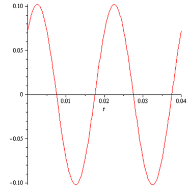
\[y(t) = \int_{-\infty}^{t} \frac{d\varphi(\theta)}{d\theta} f(t – \theta) d\theta. \tag{33}\]
The obtained results are independent on the reference frame and the origin of time measuring. This means that the description is objective in sense of Galileo-Newton-Einstein. Moreover, the presented descriptions are consistent. Remark also the place where the ’power’ laws were incorporated (right hand members) and the time dependent derivative of ’sizes’ is not affected.
The von Schweidler current for \(\beta=0.013\), \(C=0.25\), \(n=-0.5\), and \(\phi(\theta)=\sin(100\pi\theta)\) is shown in Figure 28.
In this context \(f(t)\), is the function that represents the behavior after a single step change with absolute value 1, that is, as mentioned above:
\[f(t) = \beta C t^{-n}. \tag{34}\]
Like all material constants, the constants \(\beta\) and \(n\) which determine the course of residue formation are also considered as functions of temperature. The statements of various observers (Bedell and Kinsleg; Hopkinson and Wilson; Naccari; Schweidler) concerning the influence of temperature present contradictions, which, however, may only be apparent. It is usually stated that the residue decreases with increasing temperature; other observers state that the constant \(\beta\) increases with increasing temperature, while the exponent \(n\) is not significantly influenced by temperature. From this last statement, it would follow that the residual charge formed in a given time \(\delta\) \[R=\frac{\beta \times C \times E \times t^{1-n}}{1-n}, \tag{35}\] changes with temperature.
However, if, after a longer operating time, the capacitor is momentarily discharged, one terminal is then isolated, and the residual charge, which rises to a maximum and then falls again, is measured using an electrometric method, the observed maximum may be reduced at higher temperatures, namely if the conductivity of the dielectric increases more rapidly with temperature than the magnitude of the charge. Two observations on the influence of mechanical and electrical state changes on the formation of residues are also worth mentioning.
According to Hopkinson, the abnormal charging and discharging currents in a Leyden jar are intensified by simultaneous mechanical shocks. According to Hoor the states that the formation of residues in a capacitor can be reduced by frequent “forming”, i.e. alternating charging and discharging.
In [26] authors introduce a unified fractional derivative, defined by two parameters (order and asymmetry). From this, all the interesting derivatives can be obtained. Authors reveal that ’Four centuries after the first reference to the possibility of non-integer order derivatives, the presently termed Fractional Calculus (FC) has reached a crossroads where multiple definitions are mixed, causing a huge confusion that makes life very difficult for those who only intend to make applications in Science and Engineering’. ’The number of currently existing fractional derivatives (FDs) is so high, which became the biggest obstacle to the diffusion of FC in Science and Engineering’. For reduce the possible confusions in the following we will consider only the so called Caputo and Rieman-Liouville temporal fractional order derivatives and we will show why the use of these derivatives are inappropriate in the description of real word phenomena.
For a continuously differentiable function \(f: [0,\infty) \rightarrow \mathbb{R}^{1}\), the Caputo fractional derivative of order \(\alpha\), \(0 < \alpha < 1\) is defined with formula:
\[\label{eq36} D_{C}^{\alpha}f(t) = \frac{1}{\Gamma(1-\alpha)} \int_{0}^{t} \frac{f'(\tau)}{(t-\tau)^{\alpha}} d\tau. \tag{36}\]
For a continuously differentiable function \(f: [0,\infty) \rightarrow \mathbb{R}^{1}\), the Riemann-Liouville fractional derivative of order \(\alpha\), \(0 < \alpha < 1\) is defined with formula:
\[\label{eq37} D_{R-L}^{\alpha}f(t) = \frac{1}{\Gamma(1-\alpha)} \frac{d}{dt} \int_{0}^{t} \frac{f(\tau)}{(t-\tau)^{\alpha}} d\tau. \tag{37}\]
In the paper [27], authors show that the mathematical description of mechanical movements using temporal fractional order derivatives defined by formula (36) and (37) is not objective. In [27] the material particle movement and the movement of a continuum body is treated. It is shown for example that the fractional order velocity is not objective! On the other hand, the authors of papers [28], [29] ignore complete the objectivity condition of Galileo-Newton-Einstein speaking about the fractional order velocity and theoretical basis for the application of fractional order derivatives.
In the paper [30] authors show that mathematical description of the bulk fluid flow and that of the contained impurity dispersion which uses Caputo or Riemann-Liouville fractional order partial derivatives defined by (36) and (37) is nonobjective. On the other hand, the authors of papers [31], [32] ignore complete the objectivity condition of Galileo-Newton-Einstein speaking about the applications of the temporal fractional order description of the bulk fluid flow and the contained impurity dispersion.
In the paper [33] authors show that mathematical description of the gas flow and that of the contained impurity dispersion which uses Caputo or Riemann-Liouville fractional order partial derivatives is nonobjective. On the other hand, the authors of papers [34], [35] ignore complete the objectivity condition of Galileo-Newton-Einstein speaking about the applications of the temporal fractional order description of the gas flow and the contained impurity dispersion.
In the paper [36] authors show that for guitar string, the mathematical description of strain, constitutive law, and dynamics, by direct replacement of integer order derivatives with classic Caputo or Riemann-Liouville fractional order partial derivatives is nonobjective. On the other hand, the authors of papers [37], [38], [39], [40] ignore complete the objectivity condition of Galileo-Newton-Einstein speaking about the applications of the temporal fractional order description of time fractional wave equation.
In the paper [41] authors show that Mathematical Description of the Groundwater Flow and that of the Impurity Spread, which use temporal Caputo or Riemann-Liouville fractional partial derivatives, is non-objective. On the other hand, the authors of papers [42]-[46] ignore complete the objectivity condition of Galileo-Newton-Einstein, speaking about the applications of the temporal fractional order description in groundwater flow.
In the paper [47] authors show that mathematical description of the ion transport across biological neuron membrane and in biological neuron networks, voltage propagation along neuron axons and dendrites, which uses temporal classic Caputo or Riemann-Liouville fractional partial derivatives, is non-objective. On the other hand, the authors of papers [48]-[50] ignore complete the objectivity condition of Galileo-Newton-Einstein speaking about the applications of the temporal fractional order description of ion transport across biological neuron membrane and in biological neuron networks, voltage propagation along neuron axons and dendrites.
In the Chapter 3 of the book [51] among different mathematical descriptions of ion transport through the membrane of cardiac tissue cells and through cardiac tissue a description which uses temporal classic Caputo or Riemann-Liouville fractional temporal and spatial partial derivatives appear. Authors shows that these descriptions are nonobjective. On the other hand, the authors of papers [52], [53] ignore complete the objectivity condition of Galileo-Newton-Einstein speaking about the applications of the temporal fractional order description of ion transport through the membrane of cardiac tissue cells and through cardiac tissue.
In [54] authors succeed to avoid violation of objectivity using the so called the general temporal fractional order Caputo and Rimann-Liouville respectively, defined by:
\[D_{C}^{\alpha}f(t) = \frac{1}{\Gamma(1-\alpha)} \int_{-\infty}^{t} \frac{f'(\tau)}{(t-\tau)^{\alpha}} d\tau, \tag{38}\]
\[D_{R-L}^{\alpha}f(t) = \frac{1}{\Gamma(1-\alpha)} \frac{d}{dt} \int_{-\infty}^{t} \frac{f(\tau)}{(t-\tau)^{\alpha}} d\tau. \tag{39}\]
Unfortunately, the consistency problem is not solved in this way.
In [55] authors discuss the general problem of initialized fractional calculus.
In [56] author discuss the initial conditions in continuous time fractional linear systems in signal processing.
In [57] the authors discuss the role of prehistories in the initial value problems of fractional viscoelastic equations.
In [58] the authors search an answer to the question: How to impose physically coherent initial conditions to a fractional system?
In [59] the authors make an interesting comment on the description and initialization of fractional partial differential equations using Riemann-Liouville’s and Caputo’s definitions.
In [60] the authors discuss system of initial conditions vs derivative initial conditions.
In [61] the author present interesting distributed time delay models as an alternative to fractional calculus-based models for fractional behavior modeling.
Classical mathematical models of real word phenomena are objective in sense of Galileo-Newton-Einstein i.e. are independent of the choice of reference frame and on the choice of the origin of time measuring.
The constitutive law in elasticity, fluid and gas dynamics as well the contained impurity dispersion, thermotransport, electricity and electrodynamics were incorporated successfully via the right hand member of the equation, boundary conditions and initial condition (§2.2).
New mathematical models, obtained starting from an existing classical model and changing the integer order derivatives with Caputo or Riemann-Liouville fractional order derivatives are non-objectives and are inconsistent. Therefore, they are not appropriate for describe real word phenomena (§6).
The Kepler power law in astronomy were incorporated successfully by Newton in classical model of planets dynamic by creating a new mathematical tool, termed calculus, via initial value condition (§4).
Curie-von Schweidler power law concerning the response of dielectric material to the step input of a direct current (DC) voltage were incorporated successfully, as constitutive law in the mathematical description of the current dynamics of a series RLC circuit in case of a (AC) input. The mathematical tool used in this description is not anymore a second order differential equation (§5).
In §7 there are different ideas concerning initializing and initial conditions in case of fractional order model. Unfortunately conserving the fractional order derivatives non objectivity and consistency problems are not avoided. Just the presented distributed time delay model is appropriate for that purpose.
Incorporating the power lows as the constitutive laws can be also an appropriate way.
This research received no external funding.
Data created and analyzed in this study are available on request.
The authors declare no conflict of interest.