Existence, Stability and Instability Conditions of a Static Meniscus Appearing in Dewetted Bridgman Single Crystal Cylindrical Bar Growth From Melt

1. Introduction

According to [1] “Dewetting” refers to a phenomenon that has occurred spontaneously during many experiments of Bridgman solidification of semiconductors in space (see reviews [2, 3]). It also refers to a process developed for crystal growth on Earth (see review in [4]). In both cases, the crystal is grown without interaction with the crucible, which considerably improves the structural quality of the material: less residual stresses, dislocations, spurious nucleation or twins. The origin of the gap between the crystal and the crucible comes from a small liquid meniscus at the level of the solid–liquid interface [5]. While the phenomenon is spontaneous under microgravity conditions, because of the lack of hydrostatic pressure, it has been adapted on Earth by applying on the liquid a gas pressure difference, \(p_h^n – p_c^g\), of the order of the hydrostatic pressure, in order to create and maintain the meniscus. For the geometry of the growth system and the main dimensions, angles, temperatures and pressures of interest in the process see [1]. Many experiments under microgravity have shown that the gap, which is typically smaller than 100 \(\mu\)m, is remarkably constant for several hours of growth. Similarly, dewetted crystals obtained on Earth demonstrate that, under given conditions (essentially a bad wetting of the liquid on the crucible), the crystal radius stays spontaneously constant, while it is almost impossible to get a dewetted crystal for other configurations [6, 7]. It then appears that the process is extremely stable (the grown crystal does not reattach to the crucible wall) in certain cases, while it shows high instability under others conditions. The thin gap thickness is directly linked to the meniscus shape and position which depend on capillary forces, hydrostatic and hydrodynamic pressures and heat transfer, all of them likely to fluctuate with time. Therefore, it is necessary, in order to master the growth process, to perform a dynamic stability analysis. Several mathematical descriptions of the Bridgman process have been published, all based on classical partial differential physical Eqs. (Young–Laplace, heat transfer, Navier–Stokes). Depending on the level of simplification, they extend from simplified autonomous nonlinear systems of differential equations [8] to numerical solutions of discretized partial differential equations [9, 10]. On this basis, several papers have been devoted to the study of the stability of dewetting, all based on Lyapunov’s theory as usually applied to crystal growth [8]: simple approaches considering only the capillary effect [12, 13] as well as more thorough analyses taking into account coupling between capillarity, heat transfer, and pressure fluctuations [13, 14]. However, such analyses consider the stability on an infinite time period and do not allow studying the time scale of perturbation recovery, nor the acceptable amplitude of the perturbations. In other words, there are cases where the system may be stable in the sense of Lyapunov, but it is useless in practice because the region of stability is too small or the recovery time is too long. On the contrary, the system may be unstable in the sense of Lyapunov, but it may oscillate sufficiently close to a state for which the performance is acceptable in practice. Practical stability is a mathematical concept allowing the analysis of these more complicated cases. Compared to Lyapunov’s stability (which concerns the stability of a specified solution of a single differential equation and its behaviour over an unbounded time interval), the practical stability of the system over a bounded time interval reflects better the reality because, in practice, the solidification takes place in a bounded time interval, and the interest is the behaviour along the whole process.

The present study deals with one other type of stability different from the above mentioned dynamic stability of the crystallization process. It concerns the stability or instability of an existing static meniscus i.e. the minimum of the free energy of the melt column i.e. that of the functional \(I(z)\) defined by: \[ I(z) = \int_{r_c}^{r_a} r \Big[ 1 + \sqrt{1 + (z')^2} – \frac{1}{2} \times p \times g \times z^2 + p \times z \Big] \, r \, dr; \quad z(r_c) = -h,\; z(r_a) = 0.\tag{1}\]

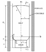
Here, \(\gamma\) is the melt surface tension; \(z = z(r)\) describes the meridian curve of the meniscus as a function of the radial coordinate \(r\) in an axis symmetric reference frame which \(Oz\) axis is directed vertically upwards (Figure 1); \(\rho\) denotes the melt density; \(g\) is the gravity acceleration, \(p = \rho \times g \times H_m – (p_c^g – p_h^g),\) denotes a pressure difference; \(H_m\) denotes the melt column height; \(H_a\) is the ampule height; \(p_c^g\) is the cold gas pressure; \(p_h^g\) is the hot gas pressure; \(r_c\) is the crystal radius; \(r_a\) is the ampule radius; \(h > 0\) is the meniscus height, \(r_a – r_c = \varepsilon\) denotes the size of the gap between the crystal and ampule walls, \(\theta_c\) is the wetting angle and \(\alpha_e\) is the growth angle.

For statically stable meniscus, indispensable (necessary) first order conditions and also second order sufficient conditions for the minimum of functional (1) should be satisfied.

The first order necessary condition is the Euler equation IS,

\[\label{eq1.2} \frac{d}{dr} \left( \frac{\partial F}{\partial z'} \right) – \left( \frac{\partial F}{\partial z} \right) = 0, \tag{2}\] where \[\label{eq1.3} F(r,z,z') = \{\gamma \times [1 + \sqrt{1 + (z')^2} + \tfrac{1}{2} \times \rho \times g \times z^2 + p \times z ] \times r, \tag{3}\] which leads to the Young–Laplace capillary equation:

\[\label{eq1.5} z'' = \frac{p – \rho g \times z}{\gamma} \times \sqrt{(1 + z'^2)^3} – \frac{1}{r} \times [1 + z'^2] \times z' \qquad \text{for } 0 < r_c \leq r \leq r_a. \tag{4}\]

As the Young–Laplace equation in hydrostatic approximation (4) is a second order differential equation formulation of boundary conditions requires assignment of two boundary conditions; one of the melt crystal interface, the second one at the melt and ampule wall interface. These conditions are: solution \(z = z(r)\) of Eq. (4) satisfy the following boundary conditions:

\[z'(r_c) = \tan\!\left(\tfrac{\pi}{2} – \alpha_e\right), \quad z'(r_a) = \tan(\theta_c – \tfrac{\pi}{2}), \quad z(r_c) = -h, \quad z(r_a) = 0,\] and

\[\label{eq1.6} z(r) \; \text{is strictly monotone on } [r_c, r_a]. \tag{5}\]

The second order sufficient conditions for the minimum of functional (1) are the Legendre condition and the Jacobi condition [15].

The Legendre condition is \[\frac{\partial^2 F}{\partial z' \partial z'} > 0. \label{eq1.7} \tag{6}\]

The Jacoby condition concerns the so-called Jacoby equation:

\[\left[ \frac{\partial^{2}F}{\partial z \, \partial z} – \frac{d}{dr} \left( \frac{\partial^{2}F}{\partial z \, \partial z'} \right) \right] \times \eta – \frac{d}{dr} \left[ \frac{\partial^{2}F}{\partial z' \, \partial z'} \times \eta' \right] = 0. \label{eq1.8} \tag{7}\]

Jacobi requirement of stability is that the solution of Eq. (7) which verifies the initial condition \(\eta(r_c) = 0\) and \(\eta'(r_a) = 1\) vanishes at most once on the interval \([r_c, r_a]\). Jacobi requirement of instability is that the solution of Eq. (7) which verifies the initial condition \(\eta(r_a) = 0\) and \(\eta'(r_a) = 1\) vanishes at least twice on the interval \([r_c, r_a]\). These conditions are sufficient conditions and can be investigated researching Sturm type upper bound or Sturm type lower bond equations for Eq. (7).

2. Existence, stability or instability of a convex meniscus

A meniscus is convex if \(z''(r) > 0\) for \(r_c \leq r \leq r_a\). Remark first that in case of a convex meniscus the function \(z'(r)\) is increasing. In particular this means that \(z'(r_c) < z'(r_a)\). Hence \(\tan\left(\frac{\pi}{2} – \alpha_e\right) < \tan(\theta_c – \tfrac{\pi}{2}), \quad \pi – \alpha_e < \theta_c – \tfrac{\pi}{2}.\) Therefore \(\pi < \alpha_e + \theta_c\).

Using the Young–Laplace capillary Eqs. (4), conditions (5) and condition \(z''(r) > 0\) for \(r_c \leq r \leq r_a\), the following result can be established:

Statement 2.1. If \(\pi < \alpha_e + \theta_c\), then a necessary condition for the existence of a function \(z(r)\) having the properties (4), (5) and \(z''(r) > 0\) for \(r_c \leq r \leq r_a\) is that the pressure difference \(p = \rho \times g\times H_m – (p_c^g – p_h^g),\) verifies:

\[\begin{aligned} &\gamma \times \frac{\alpha_{e} + \theta_{c} – \pi}{r_{a} – r_{c}} \times \sin \theta_{c} – \rho \times g \times (r_{a} – r_{c}) \times \tan\!\left(\theta_{c} – \tfrac{\pi}{2}\right) + \frac{\gamma}{r_{a}} \times \cos \alpha_{e} \notag\\ & \qquad\leq p \leq \;\; \gamma \times \frac{\alpha_{e} + \theta_{c} – \pi}{r_{a} – r_{c}} \times \sin \alpha_{e} – \frac{\gamma}{r_{c}} \times \cos \theta_{c}. \label{eq2.1} \end{aligned} \tag{8}\]

Therefore, if the pressure difference \(p = \rho g H_m – (p_c^g – p_h^g)\) a convex static meniscus exists, then the pressure difference belongs to the interval \(\left[ L_{\text{left}} \leq p \leq L_{\text{right}}\right]\), where \[ L_{\text{left}} = \gamma \frac{\alpha_e + \theta_c – \pi}{r_a – r_c} \times \sin \theta_c – \rho g \times (r_a – r_c) \times \tan(\theta_c – \tfrac{\pi}{2}) + \frac{\gamma}{r_a} \cos \alpha_e, \label{eq2.2}\ \tag{9}\] \[L_{\text{right}} = \gamma \frac{\alpha_e + \theta_c – \pi}{r_a – r_c} \times \sin \alpha_e – \frac{\gamma}{r_c} \cos \theta_c. \label{eq2.3} \tag{10}\]

In terms of the gap size \(\varepsilon = r_a – r_c\), equalities (10) and (11) can be written in the form:

\[ L_{\text{left}}(\varepsilon) = \gamma \frac{\alpha_e + \theta_c – \pi}{\varepsilon} \times \sin \theta_c – \rho g \times \varepsilon \times \tan(\theta_c – \tfrac{\pi}{2}) + \frac{\gamma}{r_a} \cos \alpha_e, \label{eq2.4}\ \tag{11}\] \[L_{\text{right}}(\varepsilon) = \gamma \frac{\alpha_e + \theta_c – \pi}{\varepsilon} \times \sin \alpha_e – \frac{\gamma}{r_a-\varepsilon} \cos \theta_c. \label{eq2.5} \tag{12}\]

For,

\[\label{eq2.6} p < L_{\text{left}}(\varepsilon), \quad \text{and} \quad p > L_{\text{right}}(\varepsilon), \tag{13}\] convex static meniscus like in Figure 1 with gap size \(\varepsilon\) does not exist.

If \(p = \rho g H_m – (p_c^g – p_h^g)\) is in the range defined by (14), convex static meniscus cannot be obtained experimentally because it collapse during the experiment.

For the existence of convex static meniscus, beside the equalities (11), (12), the next theoretical result is useful.

Statement 2.2. [16] If \(\pi < \alpha_e + \theta_c\), and \(0 < \varepsilon' < r_a\), then a sufficient condition for the existence of a number \(\varepsilon\) verifying \(0 < \varepsilon < \varepsilon'\), and the existence of a function \(z(r)\) having the properties (5) and \(z''(r) > 0\) for \(r \in [r_c, r_a]\) (i.e., convex meridian curve) is, that the pressure difference \(p = \rho g H_m – (p_c^g – p_h^g)\) verify:

\[p > \gamma \times \frac{\alpha_{e} + \theta_{c} – \pi}{\varepsilon'} \times \sin \alpha_{e} – \frac{\gamma}{r_{a} – \varepsilon'} \times \cos \theta_{c} = L_{\text{right}}(\varepsilon'). \tag{14}\]

Numerical computations were performed for the determination of a convex GaSb static meniscus. A GaSb (Gallium Antimonide) laser is a type of semiconductor laser that uses a GaSb-based material as its active region. These lasers are particularly useful for emitting light in the mid-infrared region of the spectrum, around \(2\,\mu m\), which is relevant for various applications like medical diagnostics, environmental sensing, and free-space optical communication.

The following numerical data were considered: \(r_a = 5.5 \times 10^{-3}\,[m]\), \(r_c = 5.485 \times 10^{-3}\,[m]\), \(\varepsilon = 1.5 \times 10^{-5}\,[m]\),

\(\theta_c = 2.791\,[rad]\), \(\alpha_e = 0.540\,[rad]\), \(\rho = 6.060 \times 10^{3}\,\left[\tfrac{kg}{m^3}\right]\), \(\gamma = 4.5 \times 10^{-1}\,\left[\tfrac{N}{m}\right]\), \(g = 9.81 \,\left[\tfrac{m}{s^2}\right]\), \(H_m = 60 \times 10^{-3}\,[m]\).

Computation shows that for the considered numerical data, equalities (9), (10) become: \(L_{\text{left}}(\varepsilon) = -907.882076 \,[Pa], \qquad L_{\text{right}}(\varepsilon) = -48.153047 \,[Pa].\) Therefore, in this case the pressure difference \(p = \rho\times g\times H_m – (p_c^g – p_h^g)\) has to verify: \[-907.882076 < \rho g H_m – (p_c^g – p_h^g) < -48.153047.\]

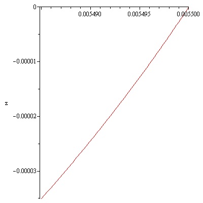
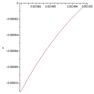
For identifying a convex static GaSb meniscus Statement 2.1 with \(\varepsilon' = 1.4862240629 \times 10^{-3}\,[\text{m}]\) was used. It was found that: \(L_{\text{right}}(\varepsilon') = 134.7790490\,[\text{Pa}]\) and for \(\varepsilon = 1.5 \times 10^{-5}\,[\text{m}]\), \(p = 1345.1652\,[\text{Pa}]\) a GaSb meniscus having convex meridian curve is obtained. The gap size of meniscus is \(\varepsilon = 1.5 \times 10^{-5}\,[\text{m}]\) and the meniscus height is \(h = 3.35 \times 10^{-5}\,[\text{m}]\). This result can be obtained by solving the following initial value problem:

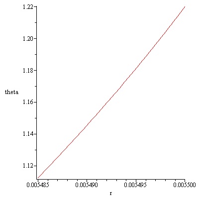
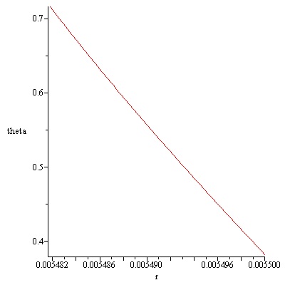
\[\frac{dz}{dr} = \tan \theta,\] \[\frac{d\theta}{dr} = \frac{-6.060 \times 10^{3} \times 9.81 \times z + 1345.1652}{4.5 \times 10^{-1}} \times \frac{1}{\cos \theta} – \frac{1}{r} \times \tan \theta,\] \[z(r_a) = 0 , \qquad \theta(r_a) = 2.791 – \frac{\pi}{2}.\] GaSb laser is shown in Figure 2. The shape of the obtained GaSb meniscus and the variation of \(\theta\) are represented in the next Figures 3 and 4.

Note that the above GaSb static meniscus was obtained by computation. This does not imply that it can be realized experimentally. For the practical creation of the above meniscus it is necessary to show that in this case the second order sufficient conditions of stability are verified.

The Legendre condition (6):

\[\frac{\partial^2 F}{\partial z'^2} > 0,\] in this case becomes

\[\frac{\partial^2 F}{\partial z'^2} = \frac{\gamma r}{(1+(z')^2)^{3/2}} > 0. \label{eq2.7} \tag{15}\]

Therefore, the Legendre condition is verified.

The Jacoby Eq. (7):

\[\left[ \frac{\partial^2 F}{\partial z' \partial z'} – \frac{d}{dr}\left(\frac{\partial^2 F}{\partial z \partial z'}\right) \right] \eta – \frac{d}{dr} \left[ \frac{\partial^2 F}{\partial z' \partial z'} \times \eta' \right] = 0,\] in this case becomes

\[\frac{d}{dr} \left[ \frac{\gamma r}{(1+(z')^2)^{3/2}} \times \eta' \right] – g \rho \times r \times \eta = 0. \label{eq2.8} \tag{16}\]

Jacobi requirement of stability condition is that the solution of Eq. (16) which verifies the initial condition \(\eta(r_a) = 0\) and \(\eta'(r_a) = 1\) vanishes at most once on the interval \([r_c, r_a]\).

In order to find a sufficient condition for Jacobi requirement, according to [10], it is sufficient to find a Sturm type upper bound for the Eq. (16).

Remark that for the coefficients of (16) in case of a GaSb static convex meniscus the following inequalities hold:

\[\frac{\gamma r}{(1+(z')^2)^{3/2}} > r_c \times \gamma \times \left(\cos(\theta_c – \tfrac{\pi}{2})\right)^3 \quad \text{and} \quad – g \rho \times r < – g \rho \times r_c. \label{eq2.9} \tag{17}\]

Hence

\[(\mu' \times r_c \times \gamma \times \left(\cos(\theta_c – \tfrac{\pi}{2})\right)^3 )' – g \rho \times r_c \times \mu = 0 \quad \text{or} \quad \mu'' = \frac{g \rho}{\gamma \times \left(\cos(\theta_c – \tfrac{\pi}{2})\right)^3}, \label{eq2.10} \tag{18}\] is a Sturm–type upper bound for (16). Remark that an arbitrary solution of (18) is given by

\[\mu(r) = A \times \sin(\omega \times r + \varphi), \label{eq2.11} \tag{19}\] where \(A\) and \(\varphi\) are real constants and

\[\omega^2 = \frac{g \rho}{\gamma \times (\sin \theta_c)^3}. \label{eq2.12} \tag{20}\]

The half period of a non-zero solution \(\mu(r)\) defined by (19) is given by

\[\frac{\pi}{\omega} = \pi \times \sqrt{\frac{\gamma \times (\sin \theta_c)^3}{g \rho}}. \label{eq2.13} \tag{21}\]

If the half period given by (21) verifies inequality

\[\frac{\pi}{\omega} = \pi \times \sqrt{\frac{\gamma \times (\sin \theta_c)^3}{g \rho}} > r_a – r_c = \varepsilon, \label{eq2.14} \tag{22}\] then the function \(\mu(r)\) defined by (19) vanishes at most once on the interval \([r_c, r_a]\).

Hence, according to [10], the solution of Jacobi Eq. (16) which verifies \(\eta(r_a) = 0\) and \(\eta'(r_a) = 1\) has only one zero on the interval \([r_c, r_a]\). Therefore the stability condition of Jacobi is verified. In other words the computed static meniscus is stable and can be realized experimentally. Note that, because inequality (22) is a sufficient condition, the inequality

\[\pi \times \sqrt{\frac{\gamma \times (\sin \theta_c)^3}{g \rho}} < \varepsilon, \label{eq2.15} \tag{23}\] does not imply that a computed convex static meniscus is unstable.

In the considered numerical case we have

\[\pi \times \sqrt{\frac{\gamma (\sin \theta_c)^3}{g \rho}} = 0.00506547181 > \varepsilon = 1.5 \times 10^{-5}.\]

Therefore the GaSb convex static meniscus obtained by computation is stable. This means that it can be realized experimentally.

Assume now that by computation a static convex GaSb meniscus was obtained. Jacobi requirement of instability of the computed static meniscus is that the solution of Eq. (7) which verifies the initial condition \(\eta(r_a) = 0\) and \(\eta'(r_a) = 1\) vanishes at least twice on the interval \([r_c, r_a]\). Therefore, the instability condition of Jacobi is verified. This condition is a sufficient condition and can be investigated researching Sturm type lower bound for Eq. (16).

Remark that for the coefficients of (16) the following inequalities hold:

\[\frac{\gamma r}{(1+(z')^2)^{3/2}} < r_a \times \gamma \times (\sin(\alpha_e))^3, \quad – g \rho \times r > – g \rho \times r_a. \label{eq2.16} \tag{24}\]

Hence

\[(\mu' \times r_a \times \gamma \times (\sin(\alpha_e))^3)' – g \rho \times r_a \mu = 0 \quad \text{or} \quad \mu'' = \frac{g \rho}{\gamma (\sin \alpha_e)^3}, \label{eq2.17} \tag{25}\] is a Sturm–type upper bound for (16). Remark that an arbitrary solution of (25) is given by

\[\mu(r) = A \times \sin(\omega r + \varphi), \label{eq2.18} \tag{26}\] where \(A\) and \(\varphi\) are real constants and

\[\omega^2 = \frac{g \rho}{\gamma (\sin \alpha_e)^3}. \label{eq2.19} \tag{27}\]

The period of a non-zero solution \(\mu(r)\) defined by (25) is given by

\[\frac{2\pi}{\omega} = 2\pi \times \sqrt{\frac{\gamma (\sin \alpha_e)^3}{g \rho}}. \label{eq2.20} \tag{28}\]

If the period of the function \(\mu(r)\) verifies inequality:

\[2\pi \times \sqrt{\frac{\gamma (\sin \alpha_e)^3}{g \rho}} > r_a – r_c = \varepsilon \quad \text{or} \quad \varepsilon > 0.01239522211, \label{eq2.21} \tag{29}\] then the function \(\mu(r)\) vanishes at least twice on the interval \([r_c, r_a]\). It follows according to [10] that the solution of the Jacobi Eq. (2.8) which verifies \(\eta(r_a) = 0\) and \(\eta'(r_a) = 1\) vanishes at least twice on the interval \([r_c, r_a]\). Therefore, the instability condition of Jacobi is verified. In other words the computed static meniscus is unstable and can’t be realized experimentally.

For a GaSb static convex meniscus the sufficient condition of stability is

\[\varepsilon < 0.00506547181\,[m],\] and the sufficient condition of instability is \[\varepsilon > 0.01239522211\,[m].\]

It follows that we cannot give an answer to the problem of stability or instability of the computed GaSb static convex meniscus for

\[0.00506547181\,[m] < \varepsilon < 0.01239522211\,[m], \label{eq2.22} \tag{30}\]

Despite this shortcoming the obtained inequalities indicate how we should choose \(r_a\) and \(r_c\) if we want to decide on the stability or instability of the static meniscus obtained by computation. More precisely: instability of the computed convex static GaSb meniscus appear when

\[r_a > 0.01239522211\,[m], \label{eq2.23} \tag{31}\] and \[r_c < r_a – 0.01239522211. \label{eq2.24} \tag{32}\]

3. Existence, stability or instability of a concave meniscus

A meniscus is concave if \(z''(r) < 0\) for \(r_c \leq r \leq r_a\). Remark first that in case of a concave meniscus the function \(z'(r)\) is decreasing. In particular this means that \(z'(r_c) > z'(r_a)\). Hence

\[\tan\left(\frac{\pi}{2} – \alpha_e\right) > \tan(\theta_c – \tfrac{\pi}{2}), \quad \pi – \alpha_e > \theta_c – \tfrac{\pi}{2}.\]

Therefore \(\pi > \alpha_e + \theta_c\).

Using the Young–Laplace capillary Eqs. (4), conditions (5) and condition \(z''(r) < 0\) for \(r_c \leq r \leq r_a\), the following result can be established:

\[\begin{aligned} \gamma \times &\frac{(\alpha_e + \theta_c – \pi)}{\varepsilon} \sin \theta_c – \rho g \times \varepsilon \times \tan\left(\tfrac{\pi}{2} – \alpha_e\right) – \frac{\gamma}{r_a} \cos \theta_c\notag\\ &\;\; \leq p \leq \;\; \gamma \times \frac{(\alpha_e + \theta_c – \pi)}{\varepsilon} \sin \alpha_e + \frac{\gamma}{r_a-\varepsilon} \cos \alpha_e, \label{eq3.1} \end{aligned} \tag{33}\] where \(\varepsilon = r_a – r_c\).

Therefore in case of the existence of a concave static meniscus the values of the pressure difference \(p = \rho g H_m – (p_c^g – p_h^g),\) have to be researched in the interval \([L_{\text{left}}(\varepsilon), L_{\text{right}}(\varepsilon)]\), where:

\[ L_{\text{left}}(\varepsilon) = \gamma \frac{\alpha_e + \theta_c – \pi}{\varepsilon} \times \sin \theta_c – \rho g \times \varepsilon \times \tan\left(\tfrac{\pi}{2} – \alpha_e\right) – \frac{\gamma}{r_a} \cos \theta_c \label{eq3.2},\ \tag{34}\] \[L_{\text{right}}(\varepsilon) = \gamma \frac{\alpha_e + \theta_c – \pi}{\varepsilon} \times \sin \alpha_e + \frac{\gamma}{r_a-\varepsilon} \cos \alpha_e. \label{eq3.3} \tag{35}\]

For

\[p = \rho g H_m – (p_c^g – p_h^g) < L_{\text{left}}(\varepsilon), \quad p = \rho g H_m – (p_c^g – p_h^g) > L_{\text{right}}(\varepsilon), \label{eq3.4} \tag{36}\] a concave static meniscus for which the gap size \(\varepsilon\) does not exist.

In other words if \(p = \rho g H_m – (p_c^g – p_h^g)\) is in the range defined by (36) concave static meniscus with gap size \(\varepsilon\) cannot be obtained experimentally because it collapse during the experiment.

Numerical computations were performed for the determination of a convex InSb static meniscus. A GaSb (Gallium Antimonide) laser is a type of semiconductor laser that uses a GaSb-based material as its active region. InSb, or indium antimonide cylindrical bars are nanostructured materials promising applications in various electronic and optoelectronic devices. They are, elongated structures made of the compound semiconductor indium antimonide. InSb is known for its high electron mobility, narrow energy bandgap, and low effective mass, making it a suitable material for infrared detectors, high-speed devices, and magnetic sensors. Indium Antimonide cylindrical bar laser based biometric identification and body temperature detection is shown in Figure 5.

The following numerical data were considered: \(r_a = 5.5 \times 10^{-3}[m], \; r_c = 5.485 \times 10^{-3}[m], \; \varepsilon = 1.5 \times 10^{-5}[m], \; \theta_c = 1.953[rad], \)\(\; \alpha_e = 0.436[rad], \; \rho = 6.582 \times 10^{3}[kg/m^3], \; \gamma = 4.2 \times 10^{-1}[N/m], \; g = 9.81[m/s^2], \; H_m = 60 \times 10^{-3}[m]\).

Computation shows that for the considered numerical data, equalities (34), (35) become: \(L_{\text{left}}(\varepsilon) = -19525.69897 \; [Pa], \quad L_{\text{right}}(\varepsilon) = -8968.72508 \; [Pa].\) Therefore, in this case the pressure difference \(p = \rho g H_m – (p_c^g – p_h^g),\) has to verify: \[-19525.69897 \; [Pa] < p = \rho g H_m – (p_c^g – p_h^g) < -8968.72508 \; [Pa].\]

For the existence of convex static meniscus beside the equalities (34), (35) the next theoretical result is useful.

Statement 3.1. [16]

If \(\pi > \alpha_e + \theta_c\), and \(0 < \varepsilon < \varepsilon'\), then a sufficient condition for the existence of a number \(\varepsilon\) verifying \(0 < \varepsilon < \varepsilon'\), and the existence of a function \(z(r)\) having the properties (5) and \(z''(r) < 0\) for \(r \in [r_c, r_a]\) (i.e. concave meridian curve) is, that the pressure difference \(p = \rho g H_m – (p_c^g – p_h^g)\) verify: \[p < \gamma \frac{\alpha_e + \theta_c – \pi}{\varepsilon'} \sin \theta_c – \rho g \varepsilon' \tan\!\left(\tfrac{\pi}{2} – \alpha_e\right) – \frac{\gamma}{r_a} \cos \theta_c = L_{\text{left}}(\varepsilon'). \label{eq3.5} \tag{37}\]

For identifying a concave static InSb meniscus Statement 3.1 with \(\varepsilon' = 1.4862240629 \times 10^{-3}[m]\) was used. It was found that: \(L_{\text{right}}(\varepsilon') = -374.8277513 \; [Pa].\) and for \(\varepsilon = 1.5 \times 10^{-5}[m], \; p = -6500[Pa]\) an In Sb static meniscus having concave meridian curve is obtained. The gap size of meniscus is \(\varepsilon = 1.5 \times 10^{-5}[m]\) and the meniscus height is \(h = 1 \times 10^{-5}[m]\). This result can be obtained by solving the following initial value problem:

\[\frac{dz}{dr} = \tan \theta,\]

\[\frac{d\theta}{dr} = \frac{-6.582 \times 10^{3} \times 9.81 \times z – 6500}{4.2 \times 10^{-1}} \times \frac{1}{\cos \theta} – \frac{1}{r} \times \tan \theta. \label{eq3.6} \tag{38}\]

\[z(r_a) = 0, \quad \theta(r_a) = 1.953 – \frac{\pi}{2}.\]

For the gap size \(\varepsilon = 1.5 \times 10^{-5}[m]\), the value of the pressure differences \(p_c^g – p_h^g\) is \[(p_c^g – p_h^g) = \rho g H_m – p = 10374.16520 [Pa].\]

The shape of the obtained InSb meniscus and the variation of \(\theta\) are represented in the next Figures 6 and 7.

Note that the above InSb static meniscus was obtained by computation. This does not imply that it can be realized experimentally. For the practical creation of the above meniscus it is necessary to show that in this case the second order sufficient conditions of stability are verified.

The Legendre condition (6) \(\frac{\partial^2 F}{\partial z'^2} > 0,\) in this case become

\[\frac{\partial^2 F}{\partial z'^2} = \frac{\gamma r}{(1+(z')^2)^{3/2}} > 0. \label{eq3.7} \tag{39}\]

Therefore, the Legendre condition is verified.

The Jacoby Eq. (7) \(\left[ \frac{\partial^2 F}{\partial z' \partial z'} – \frac{d}{dr}\left(\frac{\partial^2 F}{\partial z \partial z'}\right) \right]\eta – \frac{d}{dr}\left[ \frac{\partial^2 F}{\partial z' \partial z'} \eta' \right] = 0,\) in this case become

\[\frac{d}{dr} \left[ \frac{\gamma r}{(1+(z')^2)^{3/2}} \times \eta' \right] – g \rho \times r \times \eta = 0. \label{eq3.8} \tag{40}\]

Jacobi requirement of stability condition is that the solution of Eq. (40) which verifies the initial condition \(\eta(r_a) = 0\) and \(\eta'(r_a) = 1\) vanishes at most once on the interval \([r_c, r_a]\).

In order to find a sufficient condition for Jacobi requirement, according to [10], it is sufficient to find a Sturm type upper bound for the Eq. (40).

Remark that for the coefficients of (40) the following inequalities hold:

\[\frac{\gamma r}{(1+(z')^2)^{3/2}} > r_c \times \gamma \times (\cos(\tfrac{\pi}{2} – \alpha_e))^3, \quad – g \rho \times r < – g \rho \times r_c. \label{eq3.9} \tag{41}\]

Hence

\[(\mu' \times r_c \times \gamma \times (\cos(\tfrac{\pi}{2} – \alpha_e))^3 )' – g \rho \times r_c \mu = 0 \quad \text{or} \quad \mu'' = \frac{g \rho}{\gamma (\sin \alpha_e)^3}, \label{eq3.10} \tag{42}\] is a Sturm–type upper bound for (40). Remark that an arbitrary solution of (42) is given by

\[\mu(r) = A \sin(\omega r + \varphi), \label{eq3.11} \tag{43}\] where \(A\) and \(\varphi\) are real constants and

\[\omega^2 = \frac{g \rho}{\gamma (\sin \alpha_e)^3}. \label{eq3.12} \tag{44}\]

The half period of a non-zero solution \(\mu(r)\) defined by (43) is given by

\[\frac{\pi}{\omega} = \pi \sqrt{\frac{\gamma (\sin \alpha_e)^3}{g \rho}}. \label{eq3.13} \tag{45}\]

If the half period given by (45) verifies inequality

\[\frac{\pi}{\omega} = \pi \sqrt{\frac{\gamma (\sin \alpha_e)^3}{g \rho}} < r_a – r_c = \varepsilon, \label{eq3.14} \tag{46}\] then the function \(\mu(r)\) defined by (43) vanishes at most once on the interval \([r_c, r_a]\).

Hence, according to [10], the solution of Jacobi Eq. (40) which verifies \(\eta(r_a) = 0\) and \(\eta'(r_a) = 1\) has only one zero on the interval \([r_c, r_a]\). Therefore the stability condition of Jacobi is verified. In other words the computed static meniscus is stable and can be realized experimentally. Note that, because inequality (46) is a sufficient condition, the inequality

\[\pi \sqrt{\frac{\gamma (\sin \alpha_e)^3}{g \rho}} > \varepsilon, \label{eq3.15} \tag{47}\] does not imply that a computed convex static meniscus is unstable.

In the considered numerical case we have \(pi \sqrt{\frac{\gamma (\sin \alpha_e)^3}{g \rho}} = 0.005206913804 > \varepsilon = 1.5 \times 10^{-5}.\) Therefore the InSb convex static meniscus obtained by computation is stable. This means that it can be realized experimentally.

Assume now that by computation a static convex meniscus was obtained. Jacobi requirement of instability of the computed static meniscus is that the solution of Eq. (7) which verifies the initial condition \(\eta(r_a) = 0\) and \(\eta'(r_a) = 1\) vanishes at least twice on the interval \([r_c, r_a]\). This condition is a sufficient condition and can be investigated researching Sturm type lower bound for Eq. (40).

Remark that for the coefficients of (40) the following inequalities hold:

\[\frac{\gamma r}{(1+(z')^2)^{3/2}} \leq r_a \gamma \times (\cos(\theta_c – \tfrac{\pi}{2}))^3, \qquad – g \rho \times r > – g \rho \times r_a. \label{eq3.16} \tag{48}\]

Hence

\[(\mu' \times r_a \gamma \times (\sin(\theta_c)^3))' – g \rho \times r_a \mu = 0 \qquad \text{or} \qquad \mu'' = \frac{g \rho}{\gamma (\sin \theta_c)^3}, \label{eq3.17} \tag{49}\] is a Sturm–type upper bound for (40). Remark that an arbitrary solution of (49) is given by

\[\mu(r) = A \sin(\omega r + \varphi), \label{eq3.18} \tag{50}\] where \(A\) and \(\varphi\) are real constants and

\[\omega^2 = \frac{g \rho}{\gamma (\sin \theta_c)^3}. \label{eq3.19} \tag{51}\]

The period of a non-zero solution \(\mu(r)\) defined by (49) is given by

\[\frac{2\pi}{\omega} = 2\pi \sqrt{\frac{\gamma (\sin \theta_c)^3}{g \rho}}. \label{eq3.20} \tag{52}\]

If the period of the function \(\mu(r)\) verifies inequality:

\[2\pi \sqrt{\frac{\gamma (\sin \theta_c)^3}{g \rho}} < r_a – r_c = \varepsilon, \label{eq3.21} \tag{53}\] then the function \(\mu(r)\) vanishes at least twice on the interval \([r_c, r_a]\). Therefore according to [10] the solution of the Jacobi Eq. (3.8) which verifies \(\eta(r_a) = 0\) and \(\eta'(r_a) = 1\) vanish at least twice on the interval \([r_c, r_a]\). Therefore, the instability condition of Jacobi is verified. In other words the computed static meniscus is unstable and can’t be realized experimentally.

In the considered numerical case for an InSb static convex meniscus the sufficient condition of stability is

\[\varepsilon < 0.005206913804 \; [m],\] and the sufficient condition of instability is

\[\varepsilon > 0.01543578729 \; [m].\]

It follows that we cannot give an answer to the problem of stability or instability of the considered InSb static concave meniscus for

\[0.005206913804\,[m] < \varepsilon < 0.01543578729\,[m]. \label{eq3.22} \tag{54}\]

Despite this shortcoming the obtained inequalities indicate how we should choose \(r_a\) and \(r_c\) if we want to decide on the stability or instability of the static meniscus obtained by computation. More precisely:

instability of a convex static InSb meniscus appear when

\[r_a > 0.01543578729\,[m], \label{eq3.23} \tag{55}\]

and

\[r_c < r_a – 0.01543578729\,[m]. \label{eq3.24} \tag{56}\]

4. Results

Necessary conditions for the existence and sufficient conditions for the stability or instability of the static meniscus (liquid bridge) appearing in the cylindrical bar single crystal growth from the melt, of predetermined sizes, by using the dewetted Bridgman growth method, are presented. Theoretical results are illustrated numerically in case of GaSb laser cylindrical bar single crystal and InSb laser single crystal growth by dewetted Bridgman method.

5. Comments and Conclusions

The main novelty in this article consists in the obtained inequalities. These represent limits for what can and cannot be achieved. Experimentally, only stable static liquid bridges can be created if they exist theoretically. Unstable static liquid bridges could exist just in computation; in reality, they collapse; therefore, they are not appropriate for crystal growth.

Authors contribution

The authors contributed equally to the realization of this work. All authors have read and agreed to the published version of the manuscript.

Funding

This research did not receive any specific grant from founding agencies in the public, commercial or not-for-profit sectors.

Data Availability Statement

The original contributions presented in the study are included in the article; further inquiries can be directed to the corresponding author.

Conflicts of Interest

The authors declare no conflicts of interest.