Astrophysicists have effectively described the rotation of the Earth with its axis tilted to the orbital plane around the Sun [1]. The Earth revolves around the Sun while also rotating on its axis, influenced primarily by the gravitational forces of the Sun and the Moon, with lesser influences from the gravitational forces of other planets [2]. This results in the periodic occurrence of equinoxes and solstices [3]. Astrophysicists have collected empirical data on the positions and changes of the seasons in the Earth’s orbit, allowing them to predict seasonal events with high accuracy [4]. Key topics in research papers include seasonal climate predictability, climate variability, and climate change [5]. Scientists describe the stable tilted position of the Earth as it rotates around the Sun by the precessional motion, which maintains its orientation in space and explains the climate changes [6]. Astrophysicists argue that climate changes occur for several reasons such as solar radiation, the Earth’s surface altitude, wind directions, geological processes, magnetic pole shifts, and asteroids’ actions that tilt the Earth’s axis, etc. All of these reasons have influences on climate change that are proved by empirical data collected by physical methods from natural objects. These interpretations are based on numerous physical properties and observational experiences of different origins in their nature, and cannot be presented by one mathematical model.
Nevertheless, there is one physical aspect that influences the Earth’s climate change that a mathematical model can describe. The rotations of the Earth around its axis and the Sun represent the subject of classical mechanics with its theory of gyroscopic effects [7]. Publications on gyroscopic effects show that the inertial torques generated by the spinning mass of an object permanently change its orientation in space. The external force applied to a spinning object causes its shift, activating inertial torques that resist the change in the object’s position. The Earth’s gyroscopic effects result in the decrease of the tilt to the orbital plane. The Earth’s inclined axis to the orbit around the Sun slowly decreases because of acting gyroscopic inertial torques [8]. This process can be described analytically based only on its gyroscope properties and can clearly show the future Earth’s climate.
Fundamental publications in classical mechanics adequately describe the rotational processes of planets; however, there is a lack of comprehensive information regarding the application of gyroscope properties [9]. Engineering mechanics textbooks explain gyroscopic effects mainly through the principles established by mathematician L. Euler, specifically focusing on the torque associated with changes in angular momentum [10]. The known simplified gyroscope theories have lacked validation through practical testing [11]. The planets in orbital rotation around the Sun are under the permanent action of inertial torque, which is a gyroscopic effect omitted in science [12]. These publications discussing the gyroscopic properties of planets remained at the level of generalisations and assumptions [13].
The derived theory of gyroscopic effects for rotating objects has revealed a more complex understanding of their physics than previously thought [7]. These gyroscopic effects arise from the interplay of inertial torques generated by the object’s rotating masses around the axes of Cartesian coordinates. The inertial torques acting around each coordinate axis comprise two centrifugal torques, one Coriolis torque, and a torque due to the change in angular momentum. The magnitudes of all torques depend on the geometries of the spinning objects. The angular velocities of the objects around their axes of rotation reflect the principles of mechanical energy conservation.
Planetary mechanics focuses on rotating objects modeled as solid spheres [14]. The Earth’s surface and inner part are mostly liquid but are accepted as solid because their masses rotate with one angular velocity. Also, the Earth’s form is close to the ellipsoid of rotation, which can be accepted as a solid sphere. Such assumptions do not cause significant differences in computing the gyroscopic effects.
Analyzing the inertial torques and the angular velocities of a spinning solid sphere around axes of rotation represented by mathematical models describes planetary motion. It clarifies the gyroscopic effects associated with orbital motion around the Sun. Table 1 [7, Appendix A] presents the fundamental principles of the gyroscopic effects of a spinning solid sphere [8].
| 1. Set of inertial torques acting on the spinning solid sphere | ||
|---|---|---|
| Generated by | Action | Equation |
| centrifugal forces | resistance | \(T_{ct} = \dfrac{5}{36} \pi^3 J \omega \omega_x\) |
| precession | ||
| Coriolis forces | resistance | \(T_{cr} = \dfrac{5}{18} \pi J \omega \omega_x\) |
| change in angular momentum | resistance | \(T_{am.i} = J \omega \omega_i\) |
| precession | \(T_{am.i} = J_d \omega_k \omega_i\) | |
| 2. Kinetic energy conservation law | ||
| Angular velocities of the spinning solid sphere of horizontal | ||
| disposition about axes of rotation: \(\omega_y = \left( \frac{5\pi^3 + 5\pi + 18}{18 – 5\pi} \right) \omega_x\) | ||
Table 1 comprises the following symbols with indices: \(\omega\) and \(\omega_i\) are the angular velocities of the spinning solid sphere about axes \(oz\) and \(i\), respectively; \(J\) and \(J_d\) are the moments of inertia of the solid sphere about its axis of rotation and the diametric line, respectively; \(T_{k.i}\) is the inertial torque generated by the centrifugal force (\(ct\)), Coriolis force (\(cr\)), and the change in angular momentum (\(am\)), about axis \(i\).
The inertial torques represented in Table 1 are generated by the sphere’s mass and are interconnected by the values of the resulting axial torques. Understanding the action of inertial torques provides broad possibilities for their application in solving gyroscopic effects in engineering and astrophysics. This manuscript explores the physics of the Earth’s orbital motion and presents mathematical models for the action of the gyroscopic torques. The tilt of the Earth’s axis diminishes continuously because of the persistent influence of gyroscopic effects, which will eventually dispose it vertically on the plane of orbital motion around the Sun. The analytical model describes the physics of the Earth’s orbital motion and enables calculation of the time for future climate stabilization.
Mathematical models for the Earth’s motion around the Sun, represented in Cartesian coordinates, are derived using the well-known analytical methods of classical mechanics, which define the inertial torques acting on a spinning object. The method of cause-and-effect relationships has allowed for a detailed analysis of the inertial forces generated by the rotating masses of the Earth. The motion of the Earth around the Sun produces the external inertial torque \(T\) acting on the Earth that generates twelve inertial torques around three axes of Cartesian coordinates [7]. The impact of this external torque \(T\) was overlooked in mechanics [12]. The inertial torques \(T_{k.i}\) generated by the rotating mass of the Earth and their actions are illustrated in Figure 1. For the analysis, the Earth is considered as a rotating solid sphere and the action of all torques and motions are presented in the coordinate system \(\Sigma oxyz\).
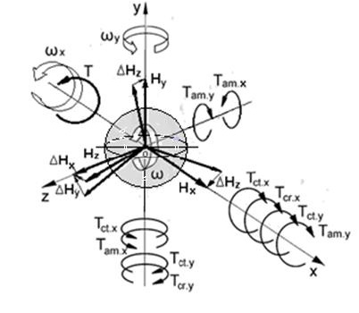
The bold and thin circular arrows, \(T\) and \(T_{k.i}\), illustrate the external and inertial torques, and the rotations around the axes. The external torque \(T\) acts counterclockwise around the axis \(ox\), generating resistance and precession torques, denoted as \(T_{k.i}\), where the index \(k\) represents the type of torque and the index \(i\) indicates the axis of action.
The tape-type circular arrows illustrate the angular velocities \(\omega_i\) of the solid sphere’s rotation around the \(ox\), \(oy\), and \(oz\) axes, all in a counterclockwise direction. The angular momentum vectors \(H_x\), \(H_y\), and \(H_z\) represent the sphere’s rotations around the respective axes. Changes in the angular momentum of the solid sphere are indicated by the vectors \(\Delta H_x\), \(\Delta H_y\), and \(\Delta H_z\) around the axes \(ox\), \(oy\), and \(oz\), respectively. These vectors represent the direction of action for the precession torques acting on the solid sphere.
The effects of inertial torques generated by the rotating mass of the sphere can be understood by analyzing the cause-and-effect relationships around the coordinate axes. A thorough examination of these torques is outlined in the following steps:
The external torque \(T\) generates two types of initial torques acting around two axes:
the resistance torques of the centrifugal \(T_{c.x} = \dfrac{5}{36} \pi^3 J \omega \omega_x\) and Coriolis \(T_{cr.x} = \dfrac{5}{18} \pi J \omega \omega_x\) forces acting around the axis \(ox\) in the clockwise direction, and
the precession torques of the centrifugal \(T_{c.x} = \dfrac{5}{36} \pi^3 J \omega \omega_x\), and the change in the angular momentum (\(\Delta H_x\)) \(T_{am.x} = J \omega \omega_x\) acting around the axis \(oy\) in the counterclockwise direction.
The effects of resistance and precession torques, along with the diagram of centrifugal forces \(f_{ct.x}\), generated by the rotating mass element \(m\) of the spinning sphere around the axes \(ox\) and \(oy\), are demonstrated in Figures 2a and 3b, respectively.
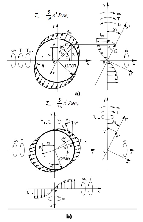
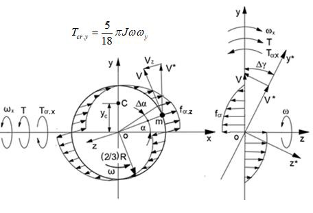
The diagram in Figure 3 demonstrates the integrated resistance Coriolis torque \[T_{cr.x} = \frac{5}{18} \pi J \omega \omega_x,\] acting in the clockwise direction around axis \(ox\) generated by the Coriolis forces \(f_{cr.x}\) of the rotating mass elements \(m\) of the spinning sphere.
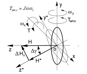
The precession torque of the change in angular momentum \[T_{am.x} = J \omega \omega_x,\] acts around the axis \(oy\) and is caused by the sphere’s center of mass. This phenomenon is well described by the renowned mathematician L. Euler. His inertial torque is considered a fundamental principle of gyroscope theory and is thoroughly documented in encyclopedias. Figure 4 illustrates the action of the torque of the change in angular momentum.
The rotation of the spinning sphere around the other axes creates inertial torques similar to those caused by centrifugal and Coriolis forces, as well as the torque resulting from changes in angular momentum. Detailed explanations of the inertial torques can be found in several publications [7, 12].
The initial inertial torques \(T_{c.x} = \dfrac{5}{36} \pi^3 J \omega \omega_x\) and \(T_{am.x} = J \omega \omega_x\), along with the load torques, generate the resistive inertial torques of the centrifugal and Coriolis forces acting around the axis \(oy\). The total torque acting around the axis \(oy\) is \[T_y = \dfrac{5}{36} \pi^3 J \omega \omega_x + J \omega \omega_x – \dfrac{5}{36} \pi^3 J \omega \omega_y – \dfrac{5}{18} \pi J \omega \omega_y.\]
The resulting torque \(T_y\) acting around the axis \(oy\) in the counterclockwise direction generates the precession torques of the centrifugal force \(T_{ct.y}\) and the torque of the change in the angular momentum (\(\Delta H_y\)), \(T_{am.y}\), acting around the axis \(ox\) in the clockwise direction. The torques \(T_{ct.y}\) and \(T_{am.y}\) are combined with the initial resistance inertial torques of the centrifugal \(T_{ct.x}\) and Coriolis \(T_{cr.x}\) torques. The total value of the resistance torques to the load torque \(T\) acting around the axis \(ox\) is \[T_{r.x} = -\frac{5}{36} \pi^3 J \omega \omega_x + \frac{5}{18} \pi J \omega \omega_x + \frac{5}{36} \pi^3 J \omega \omega_y + J \omega \omega_y.\]
The rotations of the sphere around the \(ox\) and \(oy\) axes cause changes in the angular momentum, resulting in torques \(T_{am.x} = J_x \omega_x \omega_y\) or \((\Delta H_z)\) and \(T_{am.y} = J_y \omega_y \omega_x\) or \((\Delta H_z)\), respectively. Here, \(J_{x,y} = \frac{2}{5} mR^2\) represents the moment of inertia of the sphere around its axis, while \(\omega_y\) and \(\omega_x\) denote the angular velocities of the sphere around the \(oy\) and \(ox\) axes, respectively. The precession torques \(T_{am.x}\) and \(T_{am.y}\) have equal magnitudes, act around the \(oz\) axis in opposite directions, and are mutually subtracted. They do not influence other inertial torques.
The torque \[T_x = T – \frac{5}{36} \pi^3 J \omega \omega_x – \frac{5}{18} \pi J \omega \omega_x – \frac{5}{36} \pi^3 J \omega \omega_y – J \omega \omega_y,\] acts around the axis \(ox\) and results in precession torques: the centrifugal torque \(T_{ct.x}\) and the torque of the change in angular momentum \(T_{am.x}\) acting around the axis \(oy\). These torques were initially presented as the initial ones in step 1 and are not shown in Figure 1.
The new resistive centrifugal torque \[T_{c.y} = \frac{5}{36} \pi^3 J \omega \omega_y \quad \text{and Coriolis torque} \quad T_{cr.y} = \frac{5}{18} \pi J \omega \omega_y,\] act around the \(oy\) axis, counteracting the corrected inertial torques, \(T_{c.x} = \frac{5}{36} \pi^3 J \omega \omega_x\) and \(T_{am.x} = J \omega \omega_x\).
The resulting torque \[T_y = \frac{5}{36} \pi^3 J \omega \omega_x + J \omega \omega_x – \frac{5}{36} \pi^3 J \omega \omega_y – \frac{5}{18} \pi J \omega \omega_y,\] generates the precession torques of the centrifugal force \(T_{ct.y}\) and the torque of the change in the angular momentum \(T_{am.y}\) acting around the axis \(ox\) in the clockwise direction. These torques are combined with the resistance inertial torques of the centrifugal \(T_{ct.x}\) and Coriolis \(T_{cr.x}\) torques of the axis \(ox\).
The action of the inertial torques generated by the spinning sphere is manifested by its interrelated angular velocities \[\omega_y = \left( \frac{5\pi^3 + 5\pi + 18}{18 – 5\pi} \right) \omega_x,\] around the axes according to the principle of kinetic energy conservation (Table 1).
The action of the inertial torques on the spinning sphere projects onto the Earth’s orbital motion. The Earth has an inclined axis at an angle \(\beta\). It revolves around its axis with an angular velocity \(\omega_e\), exhibiting gyroscopic properties as it rotates counterclockwise around the Sun (Figure 2) [7].
The Earth’s orbital motion generates an external inertial torque, \(T_s\), that causes the Earth to rotate synchronously about the Sun [12]. The external torque is presented by the expression \[T = J \varepsilon,\] where \(J\) is the Earth’s moment of inertia and \(\varepsilon = \omega^2\) is its angular acceleration. Here, \(\omega\) denotes the Earth’s angular velocity around the Sun, which is much smaller than \(\omega_e\) of its rotation on its axis.
The Earth’s gyroscopic effects arise from the action of inertial torques generated by the external torque \(T\) during the Earth’s orbit around the Sun. The external torque \(T\) acts on the rotating Earth, developing a set of gyroscopic torques that resist the action of \(T\). This set of gyroscopic torques is always less than the external torque \(T\), meaning that the Earth is constantly under the action of a resultant inertial torque, which gradually decreases its axial angle inclination \(\beta\).
The gyroscopic effects permanently affect the Earth, causing its axis to align perpendicularly with the orbital plane around the Sun. This decrease in the inclination of the Earth’s rotational axis resembles the behaviour of an inclined spinning top on a table. The force of gravity acting on the tilted spinning top generates gyroscopic torques that return it to a vertical position. Over time, the Earth’s axial inclination change will stabilise the climate at various latitudes.
Figure 5 illustrates the external and inertial torques acting on the Earth, along with its motions about the movable Cartesian coordinates \(\Sigma o_1 x_1 y_1 z_1\) and the fixed one around the Sun, denoted as \(\Sigma oxyz\). Circular arrows represent the inertial torques, while the Earth’s rotations around its axis and the Sun are shown using tape-like arrows. At an angle \(\beta\) from the vertical, the Earth’s tilted axis is positioned on the plane \(y_1 o z_1\) at two points during its rotation at 90 degrees, illustrating its angular momentum vectors \(H\). The graphical representation of the vectors \(H\), the action of the torques, and the Earth’s motions on the orbital plane are consistent and informative, enhancing the accompanying written explanations.
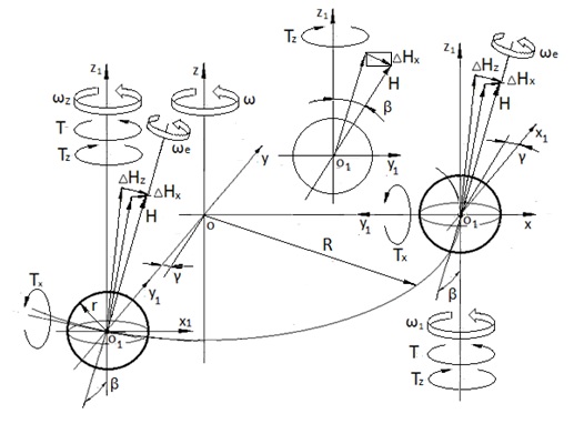
The physics of Earth’s gyroscopic torques are explained as follows. The external torque \(T\) turns the Earth’s tilt axis about a vertical axis \(o z_1\). The directions of the Earth’s rotation and its rotation by the action of the external torque coincide but do not combine because of their different physics. The external torque \(T\) turns the Earth at the angle \(\gamma\) around the axis \(oz\). The vector of the Earth’s torque of the change in angular momentum \(\Delta H_z\) about axis \(o_1 y_1 z\) acts counterclockwise around axis \(o_1 x_1\) and produces the torque of the change in angular momentum \(\Delta H_x\). The vertical component of the vector \(\Delta H_x\) acts clockwise around the axis \(o_1 z_1\) as the torque \(T_z\). The magnitude of this torque is nullified when \(\sin \beta = 0^\circ\). The horizontal component of the vector \(\Delta H_x\), \(T_x\), turns the vector \(H\) of the Earth’s axis counterclockwise around the axis \(ox\), decreases the angle \(\beta\), and produces the torque that opposes the torque \(\Delta H_z\). The gyroscopic torque \(T_x\) continuously decreases the Earth’s inclined axis in space. Consequently, the plane of the Earth, with its inclined axis, slowly shifts in space over time, and eventually, its axis will align parallel to the axis of the Sun.
The gyroscopic torques acting on the Earth generate a resultant effect that opposes the external torque \(T\). The Earth’s gyroscopic torques around the axes were described in steps 1–7 above (Figure 1–5) and Appendix A1 of reference [7]. The Earth’s resulting inertial torque \(T_x\), which accounts for the effects of centrifugal and Coriolis torques, and the change in angular momentum, causes a decrease in the angle \(\beta\) of its axis during its orbital motion around the Sun.
The equation of Earth’s relative motions around the axes in space has the following expression [7, Chapter 5]:
\[\begin{aligned} \label{eq1} (J_z + MR^2) \frac{d\omega_z}{dt} =& T – \frac{5}{36} \pi^3 J \omega_e \omega_z \sin \beta – \frac{5}{18} \pi J \omega_e \omega_z \sin \beta \notag\\ &- \left( \frac{5\pi^3 + 5\pi + 18}{18 – 5\pi} \right) J \omega_e \omega_z \sin \beta, \end{aligned} \tag{1}\]
\[\label{eq2} J_x \frac{d\omega_x}{dt} = \frac{5}{36} \pi^3 J \omega_z \omega_x \sin \beta + J \omega_z \omega_x \sin \beta – \frac{5}{18} \pi J \omega_e \omega_x \sin \beta, \tag{2}\]
\[\label{eq3} \omega_x = \left( \frac{5\pi^3 + 5\pi + 18}{18 – 5\pi} \right) \omega_z. \tag{3}\]
Transformations of Eq. (1) yield
\[\label{eq4} (J_z + MR^2) \frac{d\omega_z}{dt} = T – \left( \frac{5}{36} \pi^3 + \frac{5}{18} \pi + \frac{5\pi^3 + 5\pi + 18}{18 – 5\pi} \right) J \omega_e \omega_z \sin \beta, \tag{4}\] where all parameters are as specified above and in Table 1.
The torques acting around the axis \(o_1 z_1\) reduce the tilt of the Earth’s axis as it orbits the Sun. This effect generated by the Earth’s gyroscopic forces can be noticeable centuries later.
The Earth’s climate change depends on its tilted axis, rotation, orbital motion around the Sun and gyroscopic effects that generate all rotating objects. The influence of gyroscopic effects on the Earth’s climate is not so strong and can be noticeable centuries later. The theory of gyroscopic effects allows for calculating when the Earth’s climate is stabilized. Initial data regarding the Earth’s movements around the Sun for these calculations is represented in Table 2.
| Parameters | Dimensions | Reference |
| Mass, \( M \) | \( 5.9742 \times 10^24 \) kg | https://qntm.org/data |
| Radius, \( r \) | \( 6.3781 \times 10^6 \) m | |
| Angle of inclination to the vertical, \( \beta \) | \( 23.44^\circ \) | |
| Speed of the Earth rotation, \( \omega_e \) | \( 7.272202 \times 10^-5 \) rad/s | |
| Distance to the sun, \( R \) | \( 1.49595 \times 10^11 \) m | |
| Orbital velocity, \( V \) | 29799, 686 m/s | |
| Orbital rotation, \( \omega = V/R \) | \( 1.992024 \times 10^-7 \) rad/s | |
| Angular momentum, \( H \) | \( 7.07236 \times 10^33 \) kg m\(^2\)/s | |
| Moment of inertia \( J = (2/5)Mr^2 \) | \( 9.721256 \times 10^37 \) kg·m\(^2\) |
The external torque generated by the Earth’s turn around the Sun by the orbital motion has the following expression [12]:
\[\label{eq5} T = J \varepsilon = J \omega^2 = 9.721256 \times 10^{37} \times (1.992024 \times 10^{-7})^2 = 3.857548 \times 10^{24} \, \text{Nm}. \tag{5}\]
Substituting the defined data of Table 1 and Eq. (5) into Eq. (4) yields the following:
\[\begin{aligned} \label{eq6} &\left[9.721256 \times 10^{37} + 5.9742 \times 10^{24} \times \left(1.49595 \times 10^{11}\right)^2\right] \frac{d\omega_z}{dt}\notag\\ &\qquad = 3.857548 \times 10^{24} – \left( \frac{5}{36} \pi^3 + \frac{5}{18} \pi + \frac{5\pi^3 + 5\pi + 18}{18 – 5\pi} \right) \notag\\ &\qquad\qquad\times 9.721256 \times 10^{37} \times 7.272202 \times 10^{-5} \times \omega_z \sin 23.44^\circ. \end{aligned} \tag{6}\]
Simplification of Eq. (6) gives
\[\label{eq7} 5.431691 \times 10^{11} \frac{d\omega_z}{dt} = 1.567255 \times 10^{-11} – \omega_z. \tag{7}\]
Separating variables of Eq. (7) and transforming yield
\[\label{eq8} \frac{d\omega_z}{1.567255 \times 10^{-11} – \omega_z} = 1.841047 \times 10^{-12} \, dt. \tag{8}\]
The integral forms and transformation present Eq. (8):
\[\label{eq9} \int_0^{\omega_z} \frac{d\omega_z}{1.567255 \times 10^{-11} – \omega_z} = 1.841047 \times 10^{-12} \int_0^t dt. \tag{9}\]
The integrals of Eq. (9) are tabulated and represent the integral \[\int \frac{dx}{a – x} = -\ln|a – x| + C.\]
Solving integrals brings the following: \[\label{eq10} \ln\left(1.567255 \times 10^{-11} – \omega_z\right) \Big|_0^{\omega_z} = -1.841047 \times 10^{-12} t, \tag{10}\] giving rise to the following:
\[\label{eq11} \frac{\omega_z}{1.567255 \times 10^{-11}} = 1 – e^{-1.841047 \times 10^{-12} t}. \tag{11}\]
The right component of Eq. (11) has a small value of high order that can be neglected.
Eqs (11) and (3) give the relative angular velocities of the Earth around axes \(ox\) and \(oz\) under the action of the external torque \(T\):
\[\label{eq12} \omega_z = 1.567255 \times 10^{-11} \ \text{rad/s} = 8.979711^\circ \times 10^{-10} \ \text{/s}. \tag{12}\]
The Earth’s relative angular velocity around the axis \(oz\) Eq. (12) is less than the velocity of the orbital rotation around the Sun \(\omega = 1.992024 \times 10^{-7}\) rad/s.
\[k = \frac{\omega}{\omega_z} = \frac{1.992024 \times 10^{-7}}{1.567255 \times 10^{-11}} = 1.271027 \times 10^4.\]
The actual Earth’s angular velocity around the axis \(oz\) is
\[\omega_{ze} = \frac{\omega_z}{k} = \frac{1.567255 \times 10^{-11}}{1.271027 \times 10^4} = 1.233061 \times 10^{-15} \ \text{rad/s},\] because of the Earth’s rotation about the Sun. The angular velocity of the Earth around the axis \(ox\) is
\[\begin{aligned} \label{eq13} \omega_{xe} =& \left( \frac{5\pi^3 + 5\pi + 18}{18 – 5\pi} \right) \omega_{ze} = \left( \frac{5\pi^3 + 5\pi + 18}{18 – 5\pi} \right) \times 1.233061 \times 10^{-15}\notag\\ =& 1.015373 \times 10^{-13} \ \text{rad/s}. \end{aligned} \tag{13}\]
The direction of the Earth’s angular velocity around the axis \(ox\) Eq. (13) is in a counterclockwise (Figure 2). The time required for the Earth’s axis to turn and become parallel to the Sun’s axis is calculated using Eq. (13) by the following expression:
\[\label{eq14} t = \frac{\beta}{\omega_{xe}} = \frac{23.44^\circ}{(180^\circ/\pi)} \times \frac{1}{1.015373 \times 10^{-13}} = 4029112224448 \ \text{s} = 127762.310 \ \text{years}. \tag{14}\]
The result calculated by Eq. (14) relates only to the effects of gyroscopic torques and does not include the influence of other factors such as geological, gravitational, magnetic, and solar radiation. The gyroscopic effects change the tilt of the Earth’s rotating axis slowly in space as shown by calculating Eqs. (1)–(4). Over time, this effect will diminish when the Earth’s axis becomes perpendicular to the orbital plane.
A study of the gyroscopic effect of the Earth’s rotating axis during its orbital motion around the Sun shows slow changes in its inclination. The model depicts the Earth as a perfect solid sphere with a circular orbital trajectory. The geometry of the Earth and its orbital motion are represented by average values, which serve as the foundation for the calculations. A more accurate result would require an integration of all factors, resulting in a complex mathematical model. The inertial torque generated by the Earth’s movement around the Sun causes the planet to rotate in synchrony with its orbit in addition to its own rotation. This torque induces gyroscopic torques that act on the Earth and change its inclined axis in space. The analytical solution, the calculated data, and the graphical representations show that the Earth’s axis experiences a displacement toward the vertical position during its orbital motion. The Earth’s axis tilt is decreased, and the climate of the hemispheres will stabilise with time.
The challenges associated with the gyroscopic effects caused by the rotation of planets in the universe are intriguing aspects of astrophysics. Researchers have attempted to address these effects; however, their simplified models have not been widely adopted in publications on planetary motion. Recent studies on the theory of gyroscopic effects in rotating objects have introduced a new scientific perspective and provided a fresh analytical approach to studying planetary movements. The physics behind the gyroscopic effects of rotating planets can be explained using established principles of classical mechanics. Mathematical models that describe the inertial torques acting on the rotating Earth, which has an axis tilted relative to its orbital plane around the Sun, help clarify the physics of climate change. Additionally, the mathematical model for the Earth’s orbital motion enables predictions of climate changes and holds applied potential for astrophysics.
I would like to express my gratitude to the authorities of the Kyrgyz State Technical University after I. Razzakov for allowing me to do research as a part-time scientific staff.
All data generated or analysed during this study are included in this published article.
The author declares that the work has no conflicts of interest.
The author declares that this research received no specific grant from any funding agency in the public, commercial, or not-for-profit sectors.